Wronskian and Recurrence Formulations of QNM Conditions

The preceding page constructed four kinds of physical line: regular angular lines at the north and south axes, a future-ingoing line at the event horizon, and a selected remote radial line. A quasinormal mode (QNM) occurs when the two angular lines coincide and the two radial lines coincide at the same $(A,\omega)$. Weighted Wronskians turn those geometric intersections into two analytic equations.

A continued fraction can represent the same radial intersection in a series chart. That statement has two indispensable hypotheses: the series ansatz must synthesize the desired local endpoint line, and the minimal large-order sequence must synthesize the desired remote line. Convergence of the continued fraction by itself proves neither identification.

This page derives the coupled Wronskian formulation for scalar Kerr and the Jaffé–Leaver recurrence for scalar Schwarzschild. The numerical laboratory ends with two genuinely different checks: backward evaluation of the continued fraction and direct integration of the differential equation on an equal-magnitude ray.

First reading

Follow weighted Wronskian → angular zero → radial zero → common zero → Schwarzschild recurrence → numerical benchmark. Normalization covariance, large-order tails, exceptional strata, and AdS boundary variants may wait for a second pass.

Status ledger

Statement	Status and scope
Weighted-Wronskian and connection-entry identities	Exact for the displayed divergence-form equation
Scalar Kerr angular and flat-radial functions	Exact on Page 2’s generic subextremal sheet
Coupled common-zero and Jacobian formulas	Exact local analytic statements
Normalization invariance of zero sets	Exact for holomorphic nowhere-zero rescalings
Scalar Schwarzschild recurrence	Exact in the displayed $\ee^{-\ii\omega t}$ and $2M$ conventions
Continued fraction equals the radial QNM condition	Conditional on series synthesis and minimal-tail transfer
Scalar fundamental frequency	Converged in continued-fraction depth and cross-checked by independent ODE integration; not a rigorous enclosure
de Sitter and nonresonant AdS Wronskians	Exact once the model-specific operator and boundary line are declared
Threshold, synchronous, extremal, and resonant limits	Excluded from generic formulas and rebuilt separately
Pole of a particular Green function or correlator	Requires a numerator, domain, sheet, and normalization audit; deferred to later pages

A weighted Wronskian tests line alignment globally

Consider

$$\left(p(z)y'\right)'+q(z)y=0$$

on a connected overlap domain. With

$$\Wr[f,g]=fg'-f'g, \qquad \mathcal W_p[f,g]=p\Wr[f,g],$$

the two equations for $f$ and $g$ give

$$\frac{\dd}{\dd z}\mathcal W_p[f,g]=0.$$

Thus one evaluation in any common regular region decides whether the two solution lines coincide:

$$\mathcal W_p[f,g]=0 \quad\Longleftrightarrow\quad \operatorname{span}(f)=\operatorname{span}(g).$$

The same statement can be read as a connection-entry condition. Let

$$F=(f_1,f_2), \qquad G=(g_1,g_2), \qquad F=G\,C_{G\leftarrow F}.$$

Then

$$C_{G\leftarrow F} = \frac{1}{\mathcal W_p[g_1,g_2]} \begin{pmatrix} \mathcal W_p[f_1,g_2] & \mathcal W_p[f_2,g_2] \\ \mathcal W_p[g_1,f_1] & \mathcal W_p[g_1,f_2] \end{pmatrix}.$$

In particular, if $f_1$ and $g_2$ are the two selected vectors, their alignment is the vanishing of the $11$ entry in this ordering. Reordering $G$ changes the named entry and may change a sign, but it does not change the selected-line Wronskian. The determinant identity

$$\det C_{G\leftarrow F} = \frac{\mathcal W_p[f_1,f_2]} {\mathcal W_p[g_1,g_2]}$$

provides an immediate normalization audit.

Angular regularity defines an accessory-value sheet

For the scalar Kerr equation in $x=\cos\theta$,

$$\frac{\dd}{\dd x} \left[ (1-x^2)S' \right] + \left[ (a\omega)^2x^2 -\frac{m^2}{1-x^2} +A \right]S=0,$$

let $S_N^{\mathrm{reg}}$ and $S_S^{\mathrm{reg}}$ be the unit-leading regular vectors at $x=+1$ and $x=-1$ constructed on the preceding page. Define

$$E_{\mathrm{ang}}(A,\omega) = (1-x^2) \Wr_x \left[ S_S^{\mathrm{reg}}, S_N^{\mathrm{reg}} \right].$$

The order reversal compensates for $x=\cos\theta$ decreasing as $\theta$ increases. Equivalently,

$$E_{\mathrm{ang}} = \sin\theta\, \Wr_\theta \left[ S_N^{\mathrm{reg}}, S_S^{\mathrm{reg}} \right].$$

Either expression is independent of the match point. Its zero means that one angular solution is regular at both axes. At $a\omega=0$, smoothness gives

$$A_{\ell m}(0)=\ell(\ell+1), \qquad \ell\geq |m|.$$

Where $E_{\mathrm{ang},A}\ne0$, the implicit-function theorem and analytic continuation from this seed label an angular sheet $A_{\ell m}(a\omega)$. If $E_{\mathrm{ang}}=E_{\mathrm{ang},A}=0$, that graph chart may branch. The sheet label is part of the mode passport: merely asking a numerical angular solver for “the nearest eigenvalue” does not define continuation through such a point.

The radial endpoint pair supplies the second zero

Retain the scalar Kerr conventions

$$\begin{aligned} \Delta&=(r-r_+)(r-r_-), &K(r)&=\omega(r^2+a^2)-am,\\ \lambda&=A+a^2\omega^2-2am\omega. && \end{aligned}$$

On the generic asymptotically flat, subextremal stratum, define

$$E_{\mathrm{rad}}^{\mathrm{AF}}(A,\omega) = \Delta\Wr_r \left[ R_H^{\mathrm{in}}, R_\infty^{\mathrm{out}} \right].$$

Page 2 orders the infinity frame as

$$I= \left( R_\infty^{\mathrm{in}}, R_\infty^{\mathrm{out}} \right),$$

and its exact same-endpoint normalization is

$$\Delta\Wr_r \left[ R_\infty^{\mathrm{in}}, R_\infty^{\mathrm{out}} \right] =2\ii\omega.$$

If

$$R_H^{\mathrm{in}} = C_{\mathrm{in}}R_\infty^{\mathrm{in}} +C_{\mathrm{out}}R_\infty^{\mathrm{out}},$$

then

$$E_{\mathrm{rad}}^{\mathrm{AF}} =2\ii\omega C_{\mathrm{in}}.$$

For $\omega\ne0$, the Wronskian therefore vanishes precisely when the unwanted incoming coefficient vanishes. In the frame equation $H=I\,C_{I\leftarrow H}$, this is the $11$ entry of $C_{I\leftarrow H}$. If the infinity frame is instead ordered outgoing then incoming, the same physical condition becomes a $21$-entry zero.

The determinant audit reads

$$\det C_{I\leftarrow H} = \frac{K(r_+)}{\omega},$$

using Page 2’s horizon Wronskian $2\ii K(r_+)$. The quotient is not a formula for either $\omega=0$ or $K(r_+)=0$; both are coalescing-basis strata.

A rotating QNM is a common zero, not a radial zero

For fixed black-hole parameters and fixed integers $(\ell,m)$, the scalar Kerr QNM condition is

$$E_{\mathrm{ang}}(A,\omega)=0, \qquad E_{\mathrm{rad}}^{\mathrm{AF}}(A,\omega)=0,$$

on the declared angular and frequency sheets. A radial zero at an arbitrary value of $A$ is only one curve in $\mathbb C^2$; it is not a rotating mode. In this asymptotically flat section, abbreviate $E_{\mathrm{rad}}=E_{\mathrm{rad}}^{\mathrm{AF}}$. Likewise,

$$E_{\mathrm{ang}}E_{\mathrm{rad}}=0$$

describes the union of the two zero curves, not their intersection.

If $E_{\mathrm{ang},A}\ne0$, the implicit-function theorem gives a local sheet $A(\omega)$ with

$$A'(\omega) = -\frac{E_{\mathrm{ang},\omega}} {E_{\mathrm{ang},A}}.$$

Define the reduced radial function

$$D_{\ell m}(\omega) = E_{\mathrm{rad}} \left(A_{\ell m}(\omega),\omega\right).$$

In coordinate order $(A,\omega)$, set

$$J_{A,\omega} = \det \begin{pmatrix} E_{\mathrm{ang},A} &E_{\mathrm{ang},\omega} \\ E_{\mathrm{rad},A} &E_{\mathrm{rad},\omega} \end{pmatrix}.$$

Then

$$D_{\ell m}'(\omega) = \frac{J_{A,\omega}} {E_{\mathrm{ang},A}}.$$

A common zero with $J_{A,\omega}\ne0$ is transverse, locally isolated, and simple. If $E_{\mathrm{ang},A}=0$, the implicit-function-theorem certificate for a graph $A(\omega)$ fails; the graph may branch, or it may still exist for another reason. Keep the full two-variable system or introduce a local uniformizer. A vanishing $J$ records a non-transverse intersection; if the common zero is isolated, its local algebraic multiplicity exceeds one, while shared components are non-isolated. The Jacobian alone does not establish the geometric multiplicity data needed to diagnose an exceptional point.

When derivatives are evaluated at fixed $A$, remember that the radial coefficient uses

$$\left. \partial_\omega\lambda \right|_A =2a^2\omega-2am.$$

Normalization changes values, not genuine zero curves

Rescale the four selected vectors by holomorphic nowhere-zero functions:

$$\begin{aligned} S_N^{\mathrm{reg}}&\mapsto nS_N^{\mathrm{reg}}, &S_S^{\mathrm{reg}}&\mapsto sS_S^{\mathrm{reg}},\\ R_H^{\mathrm{in}}&\mapsto hR_H^{\mathrm{in}}, &R_\infty^{\mathrm{out}}&\mapsto oR_\infty^{\mathrm{out}}. \end{aligned}$$

The characteristic functions transform as

$$E_{\mathrm{ang}}\mapsto nsE_{\mathrm{ang}}, \qquad E_{\mathrm{rad}}\mapsto hoE_{\mathrm{rad}}.$$

Their divisors and local intersection multiplicities are unchanged. At a common zero,

$$J_{A,\omega} \mapsto nsho\,J_{A,\omega}.$$

Thus “$J$ vanishes or not” is invariant, while its numerical value is not. Characteristic derivatives and residues also retain normalization units. A Gamma factor with a zero or pole is not a unit: multiplying by it can create or erase an apparent spectral divisor.

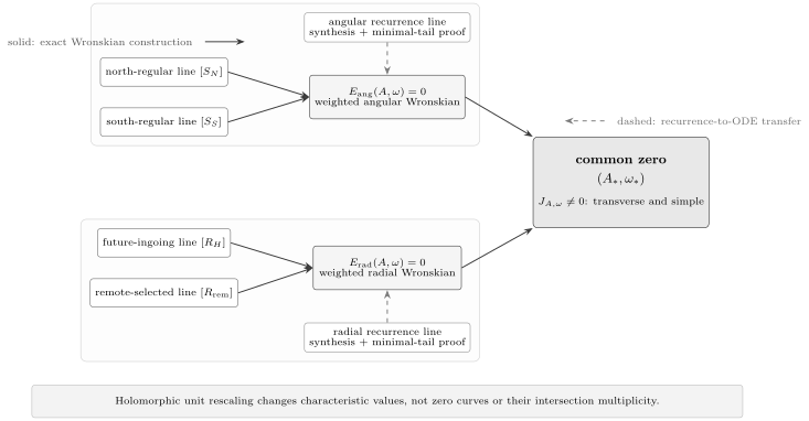
Four local physical lines produce two global alignment equations. A rotating QNM is their common zero; recurrence minimality represents the same conditions only after the synthesis and tail-transfer certificates have been established.

A recurrence is another chart on the line problem

Suppose a series ansatz converts an endpoint-normalized ODE solution into

$$\alpha_na_{n+1} +\beta_na_n +\gamma_na_{n-1}=0, \qquad n\geq0,$$

with $a_{-1}=0$. The left row selects one projective sequence line. A large-order condition—minimality in the present laboratory—selects a remote line. If $m_n$ spans that remote line, the homogeneous recurrence boundary function is

$$D_{\mathrm{rec}} = \beta_0m_0+\alpha_0m_1.$$

It remains meaningful when a ratio chart fails. On a nonsingular tail where the required $\alpha_j$ and $\gamma_j$ do not vanish and each displayed minimal-solution anchor is nonzero, Pincherle’s theorem gives

$$\frac{m_n}{m_{n-1}} = -\cfrac{\gamma_n}{ \beta_n- \cfrac{\alpha_n\gamma_{n+1}}{ \beta_{n+1}- \cfrac{\alpha_{n+1}\gamma_{n+2}}{\ddots} } }.$$

The left and minimal lines align when

$$F_{\mathrm{CF}} = \beta_0 - \cfrac{\alpha_0\gamma_1} {\beta_1- \cfrac{\alpha_1\gamma_2} {\beta_2- \cfrac{\alpha_2\gamma_3}{\ddots}}} =0.$$

This exact projective statement is developed in the Pincherle chapter. Promoting it to an ODE boundary condition requires both arrows

$$\begin{gathered} \text{left sequence line} \longleftrightarrow \text{horizon-selected ODE line}, \\ \text{minimal sequence line} \longleftrightarrow \text{remote-selected ODE line}. \end{gathered}$$

The first is a local synthesis theorem for the ansatz. The second is a large-order and endpoint-convergence theorem. A convergent continued fraction without these transfers is a sequence result, not yet a QNM result.

The scalar Schwarzschild recurrence is fully explicit

Return to the massless scalar Schwarzschild equation of the separation page. Set

$$z=\frac{r}{2M}, \qquad \Omega=2M\omega, \qquad \rho=-\ii\Omega, \qquad L=\ell(\ell+1),$$

and introduce the Jaffé coordinate

$$x=\frac{z-1}{z}.$$

The physical exterior $1<z<\infty$ maps to $0<x<1$. For the Page 1 radial unknown $\mathcal R$, use

$$\begin{aligned} \mathcal R(z) ={}& \ee^{\ii\Omega(z-1)} (z-1)^{-\ii\Omega} z^{-1+2\ii\Omega} y(x), \\ y(x) ={}& \sum_{n=0}^{\infty}a_nx^n. \end{aligned}$$

The factor $(z-1)^{-\ii\Omega}$ is future-ingoing at the horizon. The remaining powers and exponential have the outgoing phase at infinity, but the infinite series reaches the outgoing line only for its minimal coefficient sequence.

Direct substitution gives the exact core equation

$$\begin{aligned} 0={}&x(1-x)^2y'' \\ &+ \left[ 1-2\ii\Omega +(-4+8\ii\Omega)x +(3-4\ii\Omega)x^2 \right]y' \\ &+ \bigl[ 8\Omega^2+4\ii\Omega-L-1 \\ &\hspace{4.5em} +(1-4\Omega^2-4\ii\Omega)x \bigr]y. \end{aligned}$$

Equating powers of $x$, with $a_{-1}=0$ and $a_0=1$, yields

$$\alpha_na_{n+1} +\beta_na_n +\gamma_na_{n-1}=0,$$

where

$$\alpha_n =(n+1)(n+1-2\ii\Omega),$$ $$\begin{aligned} \beta_n=-\bigl[ &2n^2+(2-8\ii\Omega)n \\ &-8\Omega^2-4\ii\Omega+L+1 \bigr], \end{aligned}$$

and

$$\gamma_n=(n-2\ii\Omega)^2.$$

The seed row is

$$\alpha_0a_1+\beta_0a_0=0.$$

Writing it homogeneously is safer than dividing by $\alpha_0$, which may vanish on a resonant stratum. These coefficients agree with Leaver’s scalar recurrence after translating his Regge–Wheeler unknown and setting his $\epsilon=-1$.

For Schwarzschild, the angular condition has already fixed $A=L$. The continued-fraction equation is therefore the restriction of the coupled problem to the spherical angular sheet.

The minimal tail selects the outgoing line

Let

$$\kappa=\sqrt{-2\ii\Omega}, \qquad \operatorname{Re}\kappa>0$$

on the initial causal chart. The two formal ratio branches are

$$\frac{a_{n+1}^{(\pm)}}{a_n^{(\pm)}} = 1\pm\kappa n^{-1/2} +\left(-2\ii\Omega-\frac34\right)n^{-1} +O(n^{-3/2}),$$

and hence

$$a_n^{(\pm)} \sim n^{-\ii\Omega-3/4} \exp\!\left(\pm2\kappa\sqrt n\right).$$

The minus branch is minimal when $\operatorname{Re}\kappa>0$. Nollert uses the Fourier convention $\ee^{+\ii\omega_Nt}$ and the remainder $-a_N/a_{N-1}$; after translating $\omega_N=-\Omega$ and that extra sign, his tail is precisely the displayed expansion used as terminal data for backward continued-fraction evaluation. It accelerates a numerical representation of the same spectral condition; it is neither an additional quantization law nor, without an error analysis, a rigorous enclosure.

When $\operatorname{Re}\kappa=0$, the two generic exponentials have equal modulus and there is no Pincherle-minimal solution. Define the physical characteristic function, when possible, by an explicitly chosen lateral analytic continuation from $\operatorname{Re}\kappa>0$; analyze exact-wall polynomial or degenerate cases separately. At $\Omega=0$, even the square-root splitting collapses, in agreement with the loss of the wave basis at flat infinity.

Minimality is not polynomial truncation

A minimal solution is generally an infinite sequence subordinate to a dominant solution. A polynomial of degree $N$ instead requires

$$a_{N+1}=0, \qquad \gamma_{N+1}=0,$$

together with the finite compatibility condition from rows $0$ through $N$. Stopping a continued fraction at depth $N$ imposes a numerical tail approximation; it does not satisfy these structural termination conditions.

The spherical angular problem at $a\omega=0$ provides a genuine contrast: its regular series terminates and gives $A=\ell(\ell+1)$. A generic radial QNM Jaffé series does not terminate. Cook and Zalutskiy show that any Kerr QNM with purely imaginary frequency must be polynomial, but a polynomial solution may be a QNM, a total-transmission mode, both, or neither.

A Schwarzschild mode survives two independent tests

For the scalar fundamental mode $(\ell=0)$, evaluate the fraction backward with the plain terminal approximation $a_{N+1}/a_N=0$. Increasing the depth gives

Depth $N$	$\Omega_N=2M\omega_N$
50	$0.220884111179-0.209784913480\ii$
100	$0.220910024261-0.209792152366\ii$
200	$0.220909875786-0.209791438011\ii$
400	$0.220909878159-0.209791434171\ii$
800	$0.2209098781608394698-0.2097914341737618411\ii$
1600	$0.2209098781608393718-0.2097914341737619176\ii$
3200	$0.2209098781608393718-0.2097914341737619176\ii$
6400	$0.2209098781608393718-0.2097914341737619176\ii$

The $N=3200$ and $N=6400$ runs agree beyond the digits shown in the table. Their stabilized plain-tail value is

$$\begin{aligned} \Omega_{00} ={}& 0.220909878160839371750923012336 \\ &-0.209791434173761917563478133711\ii, \end{aligned}$$

or

$$\begin{aligned} M\omega_{00} ={}& 0.110454939080419685875461506168 \\ &-0.104895717086880958781739066855\ii. \end{aligned}$$

Depth convergence is only an internal recurrence check. For an independent ODE test, write the Regge–Wheeler unknown as $u=r\mathcal R$ and integrate the dimensionless logarithmic derivative

$$w(z)=\frac{\partial_z u}{u}.$$

For the scalar equation it obeys

$$\begin{aligned} \frac{\dd w}{\dd z} ={}&-w^2-\frac{w}{z(z-1)} -\frac{\Omega^2z^2}{(z-1)^2} \\ &+\frac{L}{z(z-1)} +\frac{1}{z^2(z-1)}. \end{aligned}$$

Reproduction data for the direct ODE check

Put $\rho=-\ii\Omega$. At the horizon, set

$$u=(z-1)^\rho \sum_{k=0}^{\infty}h_k(z-1)^k, \qquad h_0=1,$$

with $h_j=0$ for $j<0$. Direct substitution, independently of the Jaffé ansatz, gives

$$\begin{aligned} 0={}&k(k+2\rho)h_k +H_kh_{k-1}+I_kh_{k-2} \\ &-4\rho^2h_{k-3}-\rho^2h_{k-4}, \end{aligned}$$

where

$$\begin{aligned} H_k={}& 2(\rho+k-1)(\rho+k-2) +(\rho+k-1) \\ &-4\rho^2-L-1, \\ I_k={}& (\rho+k-2)(\rho+k-3) -6\rho^2-L. \end{aligned}$$

At infinity, use

$$u= \ee^{-\rho z}z^{-\rho}g(y), \qquad y=z^{-1}, \qquad g(y)=\sum_{n=0}^{\infty}c_ny^n.$$

The direct asymptotic equation is

$$\begin{aligned} 0={}&y^2(1-y)^2g'' \\ &+(y-1) \bigl[(2\rho+3)y^2-2y-2\rho\bigr]g' \\ &+\bigl[ (\rho+1)^2y^2 +(L-2\rho-1)y \\ &\hspace{4em}-(L+2\rho^2) \bigr]g. \end{aligned}$$

Equivalently, with $c_{-1}=c_{-2}=0$ and $c_0=1$,

$$2\rho(n+1)c_{n+1} +A_nc_n+B_nc_{n-1}+C_nc_{n-2}=0,$$

where

$$\begin{aligned} A_n={}&n(n-1)+(2-2\rho)n -L-2\rho^2, \\ B_n={}&-2(n-1)(n-2) -(2\rho+5)(n-1) \\ &+L-2\rho-1, \\ C_n={}&(n-2)(n-3) +(2\rho+3)(n-2) \\ &+(\rho+1)^2. \end{aligned}$$

Use continuous branches of $\operatorname{Log}(z-1)$ and $\operatorname{Log}z$ from the positive exterior into the upper-half-plane ray. The infinity vector is the lateral analytic continuation of Page 2’s causal outgoing Jost line, not a solution selected by decay on the final ray.

The horizon start uses 30 Frobenius coefficients at $z=1+10^{-5}$. The outgoing start lies at

$$z=4+T\ee^{\ii\theta}, \qquad \operatorname{Re} \left( \ii\Omega_{00}\ee^{\ii\theta} \right)=0,$$

with $\theta=43.5212526^\circ$. This equal-magnitude ray avoids the exponential ill-conditioning of real-axis inward integration. The infinity series is derived directly from the differential equation rather than from the Jaffé recurrence. At $T=40$, retain terms through $z^{-27}$, near the least term, and integrate in 64-bit arithmetic with DOP853 using relative tolerance $3\times10^{-13}$ and absolute tolerance $3\times10^{-14}$. This gives

$$w_H(4) = 0.2757594313798261 +0.2648477136298241\ii.$$

For $T=30,40,50$, changing the truncation near its least term gives

$$\left|w_H(4)-w_\infty(4)\right| <2\times10^{-10},$$

and the $T=40$ run gives $8.1\times10^{-12}$. Repeating at match points $z=3$ and $z=5$ keeps the mismatch below $2\times10^{-11}$. This is an independent residual check on physical line alignment. It does not by itself validate the 30-decimal continued-fraction value: that would require derivative-based error propagation or an enclosure. The result is an independent numerical cross-check, not an interval enclosure.

de Sitter and AdS change the remote line

The Wronskian construction is more portable than any one recurrence. For a radial equation $(p_rR')'+q_rR=0$, a black-hole event horizon and a simple cosmological horizon give

$$E_{\mathrm{rad}}^{\mathrm{dS}} = p_r\Wr \left[ R_b^{\mathrm{in}}, R_c^{\mathrm{out}} \right].$$

For scalar Schwarzschild–de Sitter, $p_r=r^2f$. The opposite signs of the event- and cosmological-horizon powers were fixed geometrically on Page 2. Kerr–de Sitter again requires this radial zero and a regular angular zero at the same accessory value.

At a nonresonant AdS boundary, write

$$R_H^{\mathrm{in}} = \alpha B_-+\beta B_+, \qquad W_0=p_r\Wr[B_-,B_+].$$

This constant is nonzero on the nonresonant stratum. If

$$p_0=\lim_{z\to0}z^{d-1}p_r(z),$$

then the unit-leading Page 2 basis gives $W_0=2\nu p_0$. Its displayed Fefferman–Graham normalization has $p_0=1$; an overall operator rescaling rescales $W_0$.

The standard line always requires a declared operator domain. The alternate and general Robin lines are available only in the admissible window $0<\nu<1$ and when the stability, unitarity, and domain conditions of the theory permit them. On such a declared domain, the three lines can be represented by

$$\begin{aligned} E_{\mathrm{std}} &= p_r\Wr[R_H^{\mathrm{in}},B_+] =\alpha W_0, \\ E_{\mathrm{alt}} &= p_r\Wr[B_-,R_H^{\mathrm{in}}] =\beta W_0, \\ E_\kappa &= p_r\Wr[R_H^{\mathrm{in}},B_-+\kappa B_+] \\ &=(\kappa\alpha-\beta)W_0. \end{aligned}$$

Thus $E_\kappa=0$ implements the explicitly declared line $\beta=\kappa\alpha$. Under $B_-\mapsto uB_-$ and $B_+\mapsto vB_+$, the same physical mixed line requires $\kappa\mapsto u\kappa/v$.

At the Breitenlohner–Freedman value $\nu=0$, the roots coalesce, $W_0=0$, and the second local vector is logarithmic. At a positive integral exponent gap, a logarithm is permitted but not forced; inspect the Frobenius obstruction and rebuild the basis only when it is present. The renormalized source/response interpretation and its scheme dependence belong to the later holographic-correlator page. More generally, an AdS QNM spectrum is not boundary-condition free: the operator domain at conformal infinity must be part of its definition.

Exceptional strata require new charts

Stratum	What fails	Required action
$\omega=0$ at flat infinity	Jost exponentials and the $2\ii\omega$ pair Wronskian collapse	Rebuild the static $r^\ell,r^{-\ell-1}$ basis and remove kinematic zeros
$K(r_+)=0$	Horizon roots collide	Use a limiting or logarithmic Levelt basis
Extremality	Two simple horizons coalesce and the Jaffé coordinate degenerates	Use Page 2’s sectorial inverse-exponential horizon vectors
$E_{\mathrm{ang},A}=0$	The implicit graph certificate fails in this chart	Retain the two-variable system; use a uniformizer if branching is present
BF value $\nu=0$	The roots coalesce and $W_0$ vanishes	Use the BF logarithmic basis and declare its renormalized boundary line
Positive integral exponent gap	A logarithm may obstruct the two-power frame	Inspect the Frobenius recursion; rebuild only when the logarithm is present
$\alpha_n=0$ or $\gamma_n=0$	A ratio chart can split or terminate	Use the homogeneous recurrence boundary function or a block recurrence
$\operatorname{Re}\sqrt{-2\ii\Omega}=0$	The generic recurrence has no Pincherle-minimal line	Declare a lateral continuation; treat exact-wall polynomial or degenerate cases separately
Continued-fraction denominator pole	The chosen projective ratio is infinite	Invert the fraction or use a Casoratian chart
$J_{A,\omega}=0$	The common zero is not transverse	Test whether it is isolated; then compute multiplicity or record a shared component

For the scalar recurrence, a particularly visible resonant set is

$$2\ii\Omega=N\in\mathbb Z_{>0},$$

where $\alpha_{N-1}=0$ and $\gamma_N=0$. This coincides with an integral horizon exponent gap. A truncated determinant or divided seed used there without a Frobenius-resonance audit is not trustworthy.

A reproducible QNM certificate has several layers

For a new black-hole equation, record the following certificate before publishing digits:

1. Convention passport. Freeze the Fourier sign, field variable, accessory definition, radial interval, branches, and analytic sheet.
2. Local-line passport. Derive each horizon, boundary, and angular line from regular coordinates or a declared boundary domain; state leading normalization and sectors.
3. Wronskian audit. Verify same-endpoint pair Wronskians, evaluate each boundary Wronskian at two match points, and check constancy.
4. Recurrence audit. Derive several rows symbolically from the ODE, retain the homogeneous seed, and identify structural coefficient zeros.
5. Tail-transfer audit. Derive the large-order branches and prove which one represents the physical remote ODE line on the chosen sheet.
6. Coupled solve. Solve both angular and radial residuals, report their scales, and evaluate $J_{A,\omega}$ rather than holding an arbitrary accessory value fixed.
7. Numerical escalation. Increase precision, series order, fraction depth, tail order, and match-point separation independently.
8. Independent method. Compare with direct ODE integration, collocation, a second recurrence chart, or a rigorously justified modern dictionary.
9. Normalization test. Rescale endpoint vectors by known analytic units and confirm that roots stay fixed while residual values transform as predicted.
10. Exceptional-stratum test. Repeat the singularity and basis audit whenever exponents, horizons, recurrence roots, or angular sheets collide.

Passing the recurrence residual alone is one layer of this certificate, not the whole certificate.

Common pitfalls

Solving only the radial equation in Kerr. A radial zero at arbitrary $A$ is a point on a radial divisor, not a QNM. Solve the angular and radial conditions together or substitute a continuously tracked angular sheet.

Calling any continued-fraction zero physical. Pincherle’s theorem identifies a minimal sequence line under its hypotheses. The ODE ansatz and large-order transfer must still identify that line with the intended horizon and remote boundary conditions.

Dividing by a collapsing pair Wronskian. Formulas such as $C_{\mathrm{in}}=E_{\mathrm{rad}}/(2\ii\omega)$ are generic-stratum quotients. At threshold, use a rebuilt static basis rather than interpreting the kinematic factor as an extra mode.

Confusing a finite fraction with a polynomial. A numerical cutoff is a tail approximation. A true polynomial additionally satisfies a structural termination condition and a finite compatibility determinant.

Exercises

1. Recover the weighted connection entry

Derive $\mathcal W_p'=0$ and the displayed formula for $C_{G\leftarrow F}$. Which entry vanishes when $f_1$ aligns with $g_2$?

Solution

For solutions $f$ and $g$,

$$\begin{aligned} \frac{\dd}{\dd z} \left[p(fg'-f'g)\right] &= f(pg')'-g(pf')' \\ &=-qfg+qgf=0. \end{aligned}$$

Write $f_1=c_{11}g_1+c_{21}g_2$. Taking weighted Wronskians with $g_2$ and with $g_1$ gives

$$c_{11} = \frac{\mathcal W_p[f_1,g_2]} {\mathcal W_p[g_1,g_2]}, \qquad c_{21} = \frac{\mathcal W_p[g_1,f_1]} {\mathcal W_p[g_1,g_2]}.$$

The second column follows identically. If $f_1$ aligns with $g_2$, then $c_{11}=0$.

2. Recover the spherical angular spectrum

Set $a\omega=0$ in the scalar angular equation. Show that the two regular axis lines align only for $A=\ell(\ell+1)$ with $\ell\geq|m|$.

Solution

The equation becomes the associated-Legendre equation

$$\frac{\dd}{\dd x} \left[(1-x^2)S'\right] + \left[A-\frac{m^2}{1-x^2}\right]S=0.$$

Factoring $(1-x^2)^{|m|/2}$ reduces it to a hypergeometric equation. A solution regular at both $x=\pm1$ exists exactly when one hypergeometric parameter is a nonpositive integer. Writing it as $-(\ell-|m|)$ gives $A=\ell(\ell+1)$ and the associated Legendre polynomial $P_\ell^{|m|}$. Therefore $E_{\mathrm{ang}}=0$ precisely on this set.

3. Identify the unwanted radial coefficient

Using Page 2’s ordered infinity pair, derive $E_{\mathrm{rad}}^{\mathrm{AF}}=2\ii\omega C_{\mathrm{in}}$. How does the named connection entry change if the infinity pair is reversed?

Solution

Insert

$$R_H^{\mathrm{in}} =C_{\mathrm{in}}R_\infty^{\mathrm{in}} +C_{\mathrm{out}}R_\infty^{\mathrm{out}}$$

into the Wronskian. Bilinearity and $\Wr[R_\infty^{\mathrm{out}},R_\infty^{\mathrm{out}}]=0$ give

$$\begin{aligned} E_{\mathrm{rad}}^{\mathrm{AF}} &= C_{\mathrm{in}} \Delta\Wr \left[ R_\infty^{\mathrm{in}}, R_\infty^{\mathrm{out}} \right] \\ &=2\ii\omega C_{\mathrm{in}}. \end{aligned}$$

With $I=(I_{\mathrm{in}},I_{\mathrm{out}})$ this is the $11$ entry of $C_{I\leftarrow H}$. With $I=(I_{\mathrm{out}},I_{\mathrm{in}})$ it is the $21$ entry.

4. Differentiate along the angular sheet

Derive $A'(\omega)$ and $D_{\ell m}'(\omega)$. Explain why $J_{A,\omega}\ne0$ is a transverse common-zero condition.

Solution

Differentiate $E_{\mathrm{ang}}(A(\omega),\omega)=0$:

$$E_{\mathrm{ang},A}A' +E_{\mathrm{ang},\omega}=0.$$

Hence $A'=-E_{\mathrm{ang},\omega}/E_{\mathrm{ang},A}$. The chain rule then gives

$$\begin{aligned} D_{\ell m}' &= E_{\mathrm{rad},\omega} -E_{\mathrm{rad},A} \frac{E_{\mathrm{ang},\omega}} {E_{\mathrm{ang},A}} \\ &= \frac{J_{A,\omega}} {E_{\mathrm{ang},A}}. \end{aligned}$$

Nonzero $J$ means the two zero curves have independent tangent covectors, so their intersection is isolated and transverse.

5. Diagnose a failed graph chart

Take

$$E_{\mathrm{ang}}=A^2-\omega, \qquad E_{\mathrm{rad}}=A-\mu.$$

Find the common zeros and show that the graph condition $E_{\mathrm{ang},A}\ne0$ can fail even when the two-variable root is simple.

Solution

The common zero is

$$(A,\omega)=(\mu,\mu^2).$$

The Jacobian in $(A,\omega)$ is

$$J = \det \begin{pmatrix} 2A&-1\\ 1&0 \end{pmatrix} =1.$$

Thus the common zero is simple for every $\mu$. At $\mu=0$, $E_{\mathrm{ang},A}=0$, so $A$ cannot be represented as a single-valued holomorphic function of $\omega$ even though the full system is regular. Using $A$ as the local parameter resolves the square-root sheet.

6. Derive the three AdS boundary functions

Starting from $R_H^{\mathrm{in}}=\alpha B_-+\beta B_+$ and $W_0=p_r\Wr[B_-,B_+]$, derive $E_{\mathrm{std}}$, $E_{\mathrm{alt}}$, and $E_\kappa$. Track the transformation of $\kappa$ under basis rescaling.

Solution

Bilinearity gives

$$p_r\Wr[R_H^{\mathrm{in}},B_+] =\alpha W_0,$$

and

$$p_r\Wr[B_-,R_H^{\mathrm{in}}] =\beta W_0.$$

For $B_\kappa=B_-+\kappa B_+$,

$$\begin{aligned} p_r\Wr[R_H^{\mathrm{in}},B_\kappa] &=\alpha\kappa W_0-\beta W_0 \\ &=(\kappa\alpha-\beta)W_0. \end{aligned}$$

If $B_-\mapsto uB_-$ and $B_+\mapsto vB_+$, the same line is represented after an irrelevant overall factor by $B_-+(u\kappa/v)B_+$. Hence $\kappa\mapsto u\kappa/v$.

7. Recover the continued-fraction sign

Starting from the three-term recurrence, derive the fraction for $m_n/m_{n-1}$ and the $n=0$ spectral residual.

Solution

Let $R_n=m_n/m_{n-1}$. Dividing row $n$ by $m_n$ gives

$$\alpha_nR_{n+1}+\beta_n+\frac{\gamma_n}{R_n}=0,$$

so

$$R_n = -\frac{\gamma_n} {\beta_n+\alpha_nR_{n+1}}.$$

Repeated substitution supplies the nested minus signs in the main text. The left row is $\beta_0m_0+\alpha_0m_1=0$, hence

$$0=\beta_0+\alpha_0R_1 = \beta_0- \frac{\alpha_0\gamma_1} {\beta_1- \dfrac{\alpha_1\gamma_2}{\beta_2-\cdots}}.$$

8. Reproduce the scalar fundamental mode

Implement backward evaluation with $R_{N+1}=0$ and solve the scalar $\ell=0$ residual near $0.22-0.21\ii$. Reproduce the $N=200,400,800$ rows and convert the stabilized value to $M\omega$.

Solution

For each trial $\Omega$, initialize $R=0$ and iterate

$$R\leftarrow -\frac{\gamma_n}{\beta_n+\alpha_nR}, \qquad n=N,N-1,\ldots,1.$$

The scalar residual is $F_N(\Omega)=\beta_0+\alpha_0R$. A complex Newton or secant solve gives

$$\begin{array}{c|c} N&\Omega_N\\ \hline 200&0.2209098757864200-0.2097914380109982\ii\\ 400&0.2209098781592576-0.2097914341708168\ii\\ 800&0.2209098781608395-0.2097914341737618\ii. \end{array}$$

Since $\Omega=2M\omega$, divide both real and imaginary parts by two to obtain the $M\omega$ value in the main text. A Nollert tail should improve convergence, but it must converge to the same root.

9. Separate truncation from minimality

Prove the two structural conditions for a degree-$N$ recurrence polynomial. Why does $R_{N+1}=0$ in a numerical fraction not prove either one?

Solution

For a degree-$N$ sequence, $a_N\ne0$ and $a_{N+1}=a_{N+2}=\cdots=0$. Rows $0$ through $N$ must admit such a vector, which is the finite compatibility or determinant condition. Row $N+1$ reduces to

$$\gamma_{N+1}a_N=0,$$

so $\gamma_{N+1}=0$. Conversely, these conditions make all later rows vanish recursively, subject to exceptional coefficient zeros being treated blockwise. A terminal value imposed only while evaluating an infinite continued fraction is discarded when $N$ is increased; it is an approximation to the remote ratio, not an identity among the recurrence coefficients.

10. Manufacture and remove a threshold zero

Suppose $E(\omega)$ is a valid characteristic function near $\omega=0$ and $E(0)\ne0$. Show how $\widetilde E=\omega E$ creates a spurious zero. Give two tests that expose it.

Solution

The zero set of $\widetilde E$ is

$$\{\omega:E(\omega)=0\}\cup\{0\}.$$

The multiplying factor is not a holomorphic unit at the origin, so divisor invariance does not apply. First, rebuild the static endpoint basis and evaluate its weighted Wronskian: it remains nonzero at the alleged root. Second, divide two nearby normalizations by their analytically known unit factors. A genuine mode is common to both reduced functions, whereas the extra factor appears only in the normalization carrying $\omega$. A direct ODE line-alignment test supplies a third check.

References

• E. W. Leaver, “An Analytic Representation for the Quasi-Normal Modes of Kerr Black Holes”, Proceedings of the Royal Society of London A 402 (1985), 285–298. Derives simultaneous angular and radial continued fractions for Kerr and the Schwarzschild recurrence used here.
• W. Gautschi, “Computational Aspects of Three-Term Recurrence Relations”, SIAM Review 9 (1967), 24–82. States Pincherle’s theorem with its minimal-solution hypotheses and develops stable recurrence computation.
• H.-P. Nollert, “Quasinormal Modes of Schwarzschild Black Holes: The Determination of Quasinormal Frequencies with Very Large Imaginary Parts”, Physical Review D 47 (1993), 5253–5258. Derives the asymptotic continued-fraction tail used to accelerate deep Schwarzschild modes.
• E. W. Leaver, “Remarks on the Continued-Fraction Method for Computing Black-Hole Quasinormal Frequencies and Modes”, Physical Review D 45 (1992), 4713–4716. Separates Jaffé-series endpoint convergence from continued-fraction convergence and identifies the absence of a minimal solution on the negative-real $\rho$ axis.
• G. B. Cook and M. Zalutskiy, “Modes of the Kerr Geometry with Purely Imaginary Frequencies”, Physical Review D 94 (2016), 104074. Shows that purely imaginary Kerr QNMs must be polynomial while polynomial solutions need not be QNMs.
• S. Dyatlov, “Quasi-Normal Modes and Exponential Energy Decay for the Kerr–de Sitter Black Hole”, Communications in Mathematical Physics 306 (2011), 119–163. Gives a rigorous scalar-wave resonance framework for sufficiently slowly rotating Kerr–de Sitter.
• C. M. Warnick, “On Quasinormal Modes of Asymptotically Anti-de Sitter Black Holes”, Communications in Mathematical Physics 333 (2015), 959–1035. Defines QNMs for globally stationary asymptotically AdS black holes through a horizon-regular generator with fixed admissible stationary boundary conditions, and proves meromorphic resolvent statements in the stated Sobolev half-planes.
• F. Novaes, C. I. S. Marinho, M. Lencsés, and M. Casals, “Kerr–de Sitter Quasinormal Modes via Accessory Parameter Expansion”, Journal of High Energy Physics 05 (2019), 033. Formulates coupled radial and angular Heun–monodromy constraints and solves them perturbatively in its small-extremality and small-rotation regimes, with separate qualifications at resonant monodromy data.