Riemann–Hilbert Problems and Character Varieties

“The Riemann–Hilbert problem” names several related but inequivalent questions. One asks which flat connection corresponds to a local system, another asks whether prescribed monodromy can be realized by a Fuchsian matrix on a chosen bundle, and a third asks for a piecewise-holomorphic matrix with specified contour jumps. Character varieties organize representation data for the first two questions; they are not themselves solutions of the third.

This page builds a firewall between those meanings, then develops two concrete tools. The first is the relative $SL(2,\mathbb C)$ character variety of the four-punctured sphere, written as an explicit Fricke cubic. The second is a normalized contour problem whose solvability is controlled by a singular integral operator or, geometrically, by partial indices.

Three questions share one historical name

Problem	Input	Requested output	Main qualification
Regular-singular correspondence	A local system or monodromy representation	A regular-singular flat connection, up to isomorphism	The underlying bundle and its extension matter
Prescribed-monodromy realization	Punctures and monodromy matrices	A Fuchsian system in a chosen global trivialization	The required logarithmic bundle may be nontrivial
Contour matrix problem	An oriented contour, jumps, local behavior, and normalization	A piecewise-holomorphic matrix with those boundary values	Compatibility does not guarantee analytic solvability

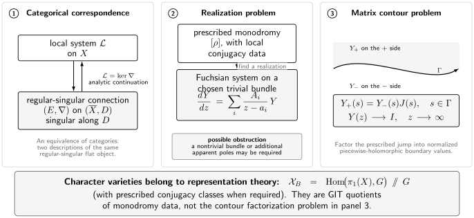
Three Riemann–Hilbert questions with different inputs and obstructions. Character varieties are GIT quotients of representation data; a contour jump problem is a separate analytic factorization problem.

Local systems and regular-singular connections

Let $X=\overline X\setminus D$, where $\overline X$ is a compact Riemann surface and $D$ is a finite set. On $X$, taking horizontal sections gives an equivalence between complex local systems and holomorphic vector bundles with flat connection. Deligne’s regular-singular correspondence gives the algebraic version: finite-dimensional local systems on $X^{\mathrm{an}}$ correspond to algebraic flat connections regular singular along $D$.

This is a categorical statement, not a formula for one preferred coefficient matrix. A representation does not by itself choose

• a global trivialization of the holomorphic bundle;
• a logarithmic lattice or extension across each point of $D$;
• a cyclic vector that turns a system into one scalar equation; or
• normalized local solution frames and their connection matrices.

Local monodromy determines residue eigenvalues only modulo integers. A Deligne extension becomes canonical after choosing representatives in a specified half-open width-one strip. Changing those logarithms by integers—equivalently, moving the strip across an eigenvalue class—can change the logarithmic extension of the same local system. Thus ordinary monodromy cannot recover all of the extension data already identified on the monodromy page.

Realizing monodromy in a prescribed trivialization

The classical system realization problem on the sphere is stronger. Given punctures $a_1,\ldots,a_{m-1},\infty$ and a representation, seek

$$\frac{\dd Y}{\dd z} = \sum_{i=1}^{m-1} \frac{A_i}{z-a_i}\,Y, \qquad A_\infty = -\sum_{i=1}^{m-1}A_i,$$

on the trivial bundle $\mathcal O_{\mathbb P^1}^{\oplus n}$, with exactly those poles and the prescribed monodromy. The categorical correspondence supplies a logarithmic connection on some holomorphic bundle. It does not assert that this bundle is trivial.

This distinction is substantive. The classical unconstrained $GL(2,\mathbb C)$ system realization problem on the sphere has a positive solution, but Bolibrukh produced a rank-three representation with four prescribed singular points that has no realization of the displayed kind. This does not imply positivity for scalar realization, prescribed logarithmic lattices, traceless lifts, or other constrained variants. Depending on the problem, one may instead permit a nontrivial bundle, alter the logarithmic extension, or add apparent singularities. Passing to a scalar equation is stricter still: a cyclic vector can introduce apparent poles even when the system itself has none.

Factoring jumps on a contour

The modern matrix problem starts from an oriented contour $\Gamma$ and a jump matrix $J$. With the $+$ side on the left, one seeks a matrix $Y$ analytic away from $\Gamma$ such that

$$Y_+(s)=Y_-(s)J(s), \qquad Y(z)=I+O(z^{-1}) \quad (z\to\infty).$$

A complete problem must also specify the function spaces, endpoint and junction behavior, allowed poles, and local normalization. Even if every $J(s)$ is invertible and all local products are compatible, a normalized solution need not exist. This is an analytic factorization problem, not merely a restatement of the categorical correspondence.

The contour problem developed below is pole-free. If poles are allowed, replace analyticity by meromorphy and prescribe every principal part or residue condition.

Representation tuples and the quotient by frames

Every matrix in the tuple below acts in one common frame at the base point $z_*$. If $D_i$ is first computed in a local frame at the $i$th puncture, the connection-matrix page transports it as

$$M_i=C_{*i}D_iC_{*i}^{-1}.$$

For an oriented genus-$g$ surface with $m$ punctures, choose based generators obeying

$$\prod_{j=1}^{g}[A_j,B_j]\, M_1M_2\cdots M_m =I, \qquad [A,B]=ABA^{-1}B^{-1}.$$

On the sphere this reduces to the book’s convention

$$M_1M_2\cdots M_m=I.$$

Fix conjugacy classes $\mathcal C_i\subset G$ for the local monodromies. The framed relative representation space is

$$\begin{aligned} \mathcal R_{\boldsymbol{\mathcal C}} = \biggl\{& (A_1,B_1,\ldots,A_g,B_g, M_1,\ldots,M_m)\\ &\in G^{2g}\times \prod_{i=1}^{m}\mathcal C_i: \prod_{j=1}^{g}[A_j,B_j] \prod_{i=1}^{m}M_i=I \biggr\}. \end{aligned}$$

Here framed means globally based: the fiber at $z_*$ has been identified with a fixed vector space. It does not mean that a flag or independent frame has been chosen at each puncture. Replacing the base frame by $h\in G$ acts on every entry by

$$M\longmapsto h^{-1}Mh.$$

If each $\mathcal C_i$ is a closed conjugacy class—for example, a semisimple class—then $\mathcal R_{\boldsymbol{\mathcal C}}$ is affine, and its coarse relative character variety is

$$\mathcal X_{\boldsymbol{\mathcal C}} = \mathcal R_{\boldsymbol{\mathcal C}} \mathbin{//}G.$$

The double slash is essential. For complex reductive $G$, it denotes the affine geometric invariant theory quotient. It retains the unique closed orbit in each orbit closure. For $GL(n)$ and $SL(n)$, closed orbits correspond to completely reducible representations; a nonclosed reducible representation and its semisimplification define the same coarse point. The quotient is therefore not the naive set of all conjugacy orbits.

A nontrivial unipotent conjugacy class is not closed. With such exact local classes, the representation locus is only locally closed. Fixing traces and taking an affine quotient instead includes its closure and can add central boundary cases. One must say whether the intended object is the exact-class locus, a quotient stack, or the affine trace fiber. The tangent-space count below still applies on a smooth locally closed exact-class quotient under the same stabilizer and transversality hypotheses.

Expected dimension on the good smooth locus

Write

$$d=\dim G, \qquad z=\dim Z(G).$$

At a nonempty good smooth tuple, assume that

1. the simultaneous stabilizer is exactly $Z(G)$; and
2. the product relation is transverse, with effective rank $d-z$.

Why is the effective rank $d-z$, not $d$? Commutators vanish in the abelianization $G/[G,G]$, while each prescribed conjugacy class fixes its central character. Once the resulting compatibility condition is met, the product map varies only in the derived directions, whose dimension for a connected reductive group is $d-z$.

Then the local complex dimension is

$$\begin{aligned} \dim_{\mathbb C} \mathcal X_{\boldsymbol{\mathcal C}} &= 2gd +\sum_{i=1}^{m}\dim\mathcal C_i -2(d-z)\\ &= (2g-2)d +\sum_{i=1}^{m}\dim\mathcal C_i +2z. \end{aligned}$$

For semisimple $G$ with finite center, the last term vanishes. A noncentral semisimple conjugacy class in $SL(2,\mathbb C)$ has dimension two, so generic fixed semisimple local classes give

$$\dim_{\mathbb C}\mathcal X_{\boldsymbol{\mathcal C}} = 6g-6+2m.$$

The four-punctured sphere consequently has complex dimension two. This is an expected dimension on the good smooth transverse locus, not a promise about reducible tuples, central local monodromy, or nongeneric trace fibers.

Trace is not always a conjugacy class

For $SL(2,\mathbb C)$, a trace different from $\pm2$ fixes a noncentral semisimple conjugacy class. At trace $2$, the identity and a nontrivial unipotent matrix have the same trace; at trace $-2$, the same ambiguity occurs after multiplication by $-I$. A trace fiber can therefore be larger than a relative variety with specified unipotent local classes.

Four punctures give the Fricke cubic

Choose the ordered sphere relation

$$ABCD=I, \qquad (A,B,C,D) =(M_0,M_t,M_1,M_\infty),$$

and define the boundary traces

$$a=\operatorname{tr} A, \quad b=\operatorname{tr} B, \quad c=\operatorname{tr} C, \quad d=\operatorname{tr} D,$$

together with the positive pair traces

$$x=\operatorname{tr}(AB), \qquad y=\operatorname{tr}(BC), \qquad z=\operatorname{tr}(AC).$$

For $A,B,C,D\in SL(2,\mathbb C)$, these seven traces obey

$$\begin{aligned} 0={}&x^2+y^2+z^2+xyz\\ &-(ab+cd)x -(bc+ad)y\\ &-(ac+bd)z\\ &+a^2+b^2+c^2+d^2 +abcd-4. \end{aligned}$$

This sign convention follows the positive traces $x,y,z$ declared above. Changing one pair-trace convention changes the cubic’s printed signs.

The basic identity behind the formula is Cayley–Hamilton in rank two:

$$V+V^{-1}=(\operatorname{tr} V)I,$$

and hence

$$\operatorname{tr}(UV)+\operatorname{tr}(UV^{-1}) =(\operatorname{tr} U)(\operatorname{tr} V).$$

Repeated use, together with $D=(ABC)^{-1}$ and $\operatorname{tr}(W^{-1})=\operatorname{tr} W$, eliminates all longer words.

The seven traces $a,b,c,d,x,y,z$ generate the $SL(2,\mathbb C)$ invariant coordinate ring for this four-puncture presentation, and the Fricke polynomial is their single defining relation. With $a,b,c,d$ fixed, it is generically an affine surface in $(x,y,z)$—not an elliptic curve. A further pair-trace constraint, Hamiltonian level set, or boundary equation may produce a curve, but that is additional data. An isomonodromic deformation instead changes puncture positions while its image in the fixed character variety remains constant.

A four-unipotent checkpoint

Take

$$A= \begin{pmatrix} 1&1\\ 0&1 \end{pmatrix}, \qquad B= \begin{pmatrix} 1&0\\ 1&1 \end{pmatrix},$$

and

$$C= \begin{pmatrix} 1&-1\\ 0&1 \end{pmatrix}, \qquad D=(ABC)^{-1} = \begin{pmatrix} 0&1\\ -1&2 \end{pmatrix}.$$

Direct multiplication gives $ABCD=I$. All four boundary traces equal two, while

$$(x,y,z)=(3,1,2).$$

The specialized cubic is

$$F(x,y,z) = x^2+y^2+z^2+xyz -8x-8y-8z+28,$$

and

$$F(3,1,2)=0.$$

The tuple is irreducible. The only invariant line of the nonidentity unipotent $A$ is $\mathbb C e_1$, whereas that of $B$ is $\mathbb C e_2$; no line is common to both. The point is smooth because

$$\frac{\partial F}{\partial z}(3,1,2) = 2z+xy-8 =-1.$$

This example also exposes the trace caveat: each displayed matrix lies in a nontrivial unipotent class, but the trace value two alone would also allow the identity.

What the coarse cubic forgets

The trace coordinates describe the affine GIT quotient. If a tuple is simultaneously upper triangular but not split, its orbit is not closed; the coarse point is the diagonal semisimplification. Extension data in the off-diagonal entries has disappeared.

Singularities of a fixed Fricke surface can be checked without slogans. They obey $F=0$ together with

$$\begin{aligned} 2x+yz-(ab+cd)&=0,\\ 2y+xz-(bc+ad)&=0,\\ 2z+xy-(ac+bd)&=0. \end{aligned}$$

Strictly polystable reducible tuples, tuples with noncentral stabilizer, failures of transversality, and degenerate boundary classes are important sources of singular points. But “singular if and only if reducible” is not a safe statement on every nongeneric trace fiber. Use the stabilizer, transversality, and gradient tests appropriate to the chosen relative problem.

A normalized contour problem

Let $\Gamma$ be an oriented, piecewise smooth contour. Assume initially that $J$ and $J^{-1}$ belong to a function class for which nontangential boundary values and Cauchy projections are defined. The formulation here is pole-free; a meromorphic version must add prescribed principal parts or residue data. The normalized matrix problem is:

1. $Y$ is analytic and invertible on $\mathbb C\setminus\Gamma$;
2. its boundary values satisfy $Y_+=Y_-J$;
3. prescribed endpoint and junction singularities are obeyed; and
4. $Y(z)=I+O(z^{-1})$ at infinity.

At a contour junction, traverse a small positive circle. Crossing an edge from its $-$ side to its $+$ side contributes $J$, while the reverse crossing contributes $J^{-1}$. For a bounded removable solution, the ordered cyclic product must be $I$. If a local factor $Y=H(z)(z-v)^T$ is prescribed instead, the product records its declared local monodromy. This compatibility test is necessary, not sufficient.

Uniqueness is easier than existence

Suppose $Y^{(1)}$ and $Y^{(2)}$ are invertible solutions with the same normalization and the same local endpoint class. Then

$$R(z) = Y^{(1)}(z) \bigl(Y^{(2)}(z)\bigr)^{-1}$$

has no jump. If every endpoint singularity of $R$ is removable, then $R$ extends to an entire matrix and tends to $I$ at infinity. Liouville’s theorem gives $R=I$.

Every hypothesis in that argument matters. It proves neither invertibility nor existence, and it fails if local pole or endpoint conditions leave nonremovable freedom.

If $\det J=1$ and the endpoint singularities of $\det Y$ are removable, then $\det Y$ has no jump and tends to one. Hence

$$\det Y\equiv1.$$

Again, this is a consequence for a solution—not an existence theorem.

Constant jumps reconstruct meromorphic coefficients

Set

$$\mathcal A(z)=Y'(z)Y(z)^{-1}.$$

On each smooth contour arc, assume that $J$ and the relevant boundary values are differentiable, as happens when they extend analytically to a neighborhood of the arc. Differentiating the jump relation then gives

$$\mathcal A_+ = \mathcal A_- +Y_-J'J^{-1}Y_-^{-1}.$$

Thus $\mathcal A$ has no contour jump when $J$ is piecewise constant. Specified endpoint behavior can then force $\mathcal A$ to be rational with prescribed poles, producing a meromorphic ODE. A variable jump generally leaves a jump in $\mathcal A$ and does not directly reconstruct one global meromorphic coefficient matrix.

The singular-integral test

Let

$$(\mathcal C f)(z) = \frac{1}{2\pi\ii} \int_\Gamma \frac{f(s)}{s-z}\,\dd s,$$

and let $\mathcal C_-$ denote its boundary value from the $-$ side. A standard ansatz is

$$Y = I+\mathcal C\!\left[\mu(J-I)\right], \qquad \mu=Y_-.$$

The jump condition becomes

$$(I-\mathcal C_J)\mu=I, \qquad \mathcal C_Jf = \mathcal C_-\!\left[f(J-I)\right].$$

For a smooth compact contour and sufficiently regular $J,J^{-1}$, take the Cauchy projections on $L^2(\Gamma)$. If $I-\mathcal C_J$ is Fredholm of index zero and its homogeneous kernel is trivial, the Fredholm alternative makes it invertible. The equation then has a unique $\mu$, and the reconstruction gives the unique normalized solution once the declared endpoint and invertibility conditions are verified. A nonzero index or a nontrivial kernel requires extra analysis. Pointwise matrix compatibility alone does none of these jobs.

Partial indices detect a hidden bundle

Take the counterclockwise unit circle, so the $+$ domain is the interior. With one fixed convention, a Birkhoff factorization has the form

$$J(z) = J_-^{-1}(z) \begin{pmatrix} z^{\kappa_1}&&0\\ &\ddots&\\ 0&&z^{\kappa_n} \end{pmatrix} J_+(z),$$

where $J_+$ and its inverse are holomorphic inside, while $J_-$ and its inverse are holomorphic outside with $J_-(\infty)=I$. The integers $\kappa_1\ge\cdots\ge\kappa_n$ are the partial indices, and

$$\sum_{j=1}^{n}\kappa_j = \operatorname{wind}_{\Gamma}\det J.$$

A normalized, pole-free, everywhere-invertible solution belongs to the canonical factorization stratum, so every partial index must vanish. Zero determinant winding controls only their sum. For example,

$$J(z) = \begin{pmatrix} z&0\\ 0&z^{-1} \end{pmatrix}$$

has $\det J=1$ but partial indices $(1,-1)$. It has no canonical normalized invertible factorization.

Geometrically, $J$ glues a holomorphic vector bundle over $\mathbb P^1$. Up to the declared transition convention, the partial indices are its Birkhoff–Grothendieck splitting degrees. The example has total degree zero but splitting type $\mathcal O(1)\oplus\mathcal O(-1)$, so the bundle is not trivial. This is the contour counterpart of the bundle obstruction in prescribed-monodromy realization.

A triangular problem solved exactly

Let $\Gamma$ be a smooth positive closed contour and let $w$ be Hölder continuous. Set

$$J(s)=I+w(s)E_{12},$$

where $E_{12}^2=0$. The Plemelj relation

$$\mathcal C_+w-\mathcal C_-w=w$$

shows that

$$Y(z)=I+(\mathcal Cw)(z)E_{12}$$

satisfies

$$Y_+=Y_-J, \qquad Y(\infty)=I, \qquad \det Y=1.$$

Indeed,

$$\begin{aligned} Y_-J &= \bigl(I+(\mathcal C_-w)E_{12}\bigr) \bigl(I+wE_{12}\bigr)\\ &= I+(\mathcal C_+w)E_{12} =Y_+. \end{aligned}$$

This elementary example displays an actual solution. It should not be mistaken for a proof that a general noncommuting matrix jump admits the same construction.

Common pitfalls

Treating Deligne’s theorem as a global matrix formula. The regular-singular correspondence allows a holomorphic bundle and does not choose a global frame. A Fuchsian matrix on the trivial bundle is extra structure.

Calling the character variety a set of conjugacy classes. The affine GIT quotient remembers closed orbits and identifies a nonclosed reducible orbit with its semisimplification. At such points it can forget extension data.

Fixing only trace at a parabolic value. Trace $\pm2$ does not distinguish $\pm I$ from a nontrivial unipotent class. State the conjugacy class when that distinction matters.

Calling the four-puncture cubic a curve. With four local traces fixed, one equation in $(x,y,z)$ is generically a complex surface. A curve appears only after an additional condition or slice.

Using determinant winding as the whole factorization test. It gives the sum of the partial indices. The degree-zero splitting $\mathcal O(1)\oplus\mathcal O(-1)$ shows why that is insufficient.

Proving uniqueness and claiming existence. The Liouville ratio argument starts with two invertible solutions in the same local class. Existence requires a separate factorization, Fredholm, or vanishing-lemma argument.

Exercises

1. Count the good-locus dimension. Derive the expected dimension of the relative character variety and specialize it to noncentral $SL(2,\mathbb C)$ classes.

Solution

The ambient space of framed tuples, before imposing the product relation, has dimension

$$2g\dim G+\sum_i\dim\mathcal C_i.$$

At a good smooth transverse point, the product relation imposes $\dim G-\dim Z(G)$ independent conditions. Simultaneous conjugation has the same orbit dimension, so

$$\begin{aligned} \dim\mathcal X_{\boldsymbol{\mathcal C}} &= 2g\dim G+\sum_i\dim\mathcal C_i\\ &\qquad{} -2\bigl(\dim G-\dim Z(G)\bigr). \end{aligned}$$

For $SL(2,\mathbb C)$, $\dim G=3$, the center is finite, and every noncentral class has dimension two. The result is

$$6g-6+2m.$$

2. Audit the four-unipotent tuple. Verify the product, all seven trace coordinates, irreducibility, and smoothness of the displayed point.

Solution

Multiplication gives

$$ABC= \begin{pmatrix} 2&-1\\ 1&0 \end{pmatrix}, \qquad (ABC)^{-1} = \begin{pmatrix} 0&1\\ -1&2 \end{pmatrix} =D.$$

Thus $ABCD=I$. Direct traces give

$$a=b=c=d=2, \qquad x=3,\quad y=1,\quad z=2.$$

Substitution gives $F(3,1,2)=0$. The unique invariant lines of $A$ and $B$ are respectively $\mathbb C e_1$ and $\mathbb C e_2$, so the tuple has no common invariant line. Finally,

$$\partial_zF(3,1,2)=-1\ne0,$$

which proves smoothness by the gradient criterion.

3. Recover the two-matrix trace identity. Use Cayley–Hamilton to prove

$$\operatorname{tr}(UV)+\operatorname{tr}(UV^{-1}) =(\operatorname{tr} U)(\operatorname{tr} V)$$

for $U,V\in SL(2,\mathbb C)$.

Solution

Cayley–Hamilton for $V$ reads

$$V^2-(\operatorname{tr} V)V+I=0.$$

Multiplication by $V^{-1}$ gives

$$V+V^{-1}=(\operatorname{tr} V)I.$$

Multiply by $U$ and take the trace:

$$\operatorname{tr}(UV)+\operatorname{tr}(UV^{-1}) =(\operatorname{tr} V)(\operatorname{tr} U).$$

Repeated application to words in $A,B,C$, together with $D=(ABC)^{-1}$, yields the Fricke polynomial.

4. Solve the triangular contour problem. Prove the displayed formula for $Y$ and explain why its determinant is one.

Solution

The Plemelj formula gives

$$\mathcal C_+w=\mathcal C_-w+w.$$

Because $E_{12}^2=0$,

$$\begin{aligned} Y_-J &= \bigl(I+(\mathcal C_-w)E_{12}\bigr) \bigl(I+wE_{12}\bigr)\\ &= I+(\mathcal C_+w)E_{12} =Y_+. \end{aligned}$$

The Cauchy transform is $O(z^{-1})$ at infinity. The matrix is upper triangular with unit diagonal, so $\det Y=1$ identically.

5. Differentiate a variable jump. Assume that $J$ and the boundary values are differentiable along a smooth contour arc. Starting from $Y_+=Y_-J$, derive the jump of $\mathcal A=Y'Y^{-1}$.

Solution

Differentiate and invert the product:

$$Y_+' = Y_-'J+Y_-J', \qquad Y_+^{-1} = J^{-1}Y_-^{-1}.$$

Therefore

$$\begin{aligned} \mathcal A_+ &= \bigl(Y_-'J+Y_-J'\bigr) J^{-1}Y_-^{-1}\\ &= \mathcal A_- +Y_-J'J^{-1}Y_-^{-1}. \end{aligned}$$

The second term vanishes for a constant jump.

6. Zero winding is not enough. Find the determinant winding and partial indices of $J(z)=\operatorname{diag}(z,z^{-1})$ on the unit circle.

Solution

The matrix is already in Birkhoff diagonal form, so its partial indices are

$$(\kappa_1,\kappa_2)=(1,-1).$$

Their sum is zero, consistently with $\det J=1$ and zero determinant winding. Since the individual indices do not vanish, the factorization is not canonical; the glued bundle has splitting type $\mathcal O(1)\oplus\mathcal O(-1)$ rather than the trivial splitting.

7. Name the problem before solving it. Classify each request:

1. recover a regular-singular flat connection from a local system;
2. realize fixed monodromy by a simple-pole matrix on $\mathcal O_{\mathbb P^1}^{\oplus n}$ with no extra poles;
3. recover $Y$ from $(\Gamma,J)$ and $Y(\infty)=I$.

For the third request, suppose its pole-free singular-integral formulation has $I-\mathcal C_J$ Fredholm of index zero with trivial homogeneous kernel. What follows?

Solution

The requests are, respectively,

1. the categorical regular-singular Riemann–Hilbert correspondence;
2. the stronger prescribed-monodromy realization problem; and
3. a normalized contour matrix Riemann–Hilbert problem.

For the third, index zero and a trivial kernel imply a trivial cokernel, so the Fredholm operator is invertible. Hence there is a unique density $\mu$. Its Cauchy reconstruction gives the unique normalized solution, provided the stipulated endpoint behavior and matrix invertibility are verified.

References

• P. Deligne, Équations différentielles à points singuliers réguliers, Lecture Notes in Mathematics 163, Springer, 1970; the IAS publication page links the original scan and a separate erratum.
• D. V. Anosov and A. A. Bolibrukh, The Riemann–Hilbert Problem, Vieweg, 1994, for prescribed-monodromy realization and its obstructions.
• W. Dekkers, “The matrix of a connection having regular singularities on a vector bundle of rank 2 on $\mathbb P^1(\mathbb C)$,” in R. Gérard and J.-P. Ramis, eds., Équations différentielles et systèmes de Pfaff dans le champ complexe, Lecture Notes in Mathematics 712, Springer, 1979, 33–43, for the unconstrained rank-two realization result.
• A. A. Bolibrukh, “The Riemann–Hilbert problem”, Russian Mathematical Surveys 45 (1990), 1–58.
• A. S. Sikora, “Character varieties”, Transactions of the AMS 364 (2012), 5173–5208, for representation schemes and GIT quotients.
• W. M. Goldman, “The symplectic nature of fundamental groups of surfaces”, Advances in Mathematics 54 (1984), 200–225, and trace coordinates on the four-holed sphere.
• A. Alekseev, A. Malkin, and E. Meinrenken, “Lie group valued moment maps”, Journal of Differential Geometry 48 (1998), 445–495, for relative moduli spaces as group-valued reductions.
• S. Maloni, F. Palesi, and S. P. Tan, “On the character variety of the four-holed sphere”, Groups, Geometry, and Dynamics 9 (2015), 737–782, for the exact Fricke convention used here.
• P. Boalch and R. Paluba, “Symmetric cubic surfaces and $G_2$ character varieties”, Journal of Algebraic Geometry 25 (2016), 607–631, for cubic character varieties and quotient geometry.
• K. F. Clancey and I. Gohberg, Factorization of Matrix Functions and Singular Integral Operators, Birkhäuser, 1981, for partial indices and matrix factorization.
• P. Deift, Orthogonal Polynomials and Random Matrices: A Riemann–Hilbert Approach, AMS, 2000, for normalized contour problems and singular-integral methods.
• H. Yamane, “Riemann–Hilbert factorization of matrices invariant under inversion in a circle”, Proceedings of the AMS 147 (2019), 2147–2157, for partial-index arguments under its stated inversion-symmetry and positivity hypotheses.