Connection Coefficients as Wronskian Ratios

Wronskian matching is coordinate extraction in a two-dimensional solution space. Continue two normalized frames to one common branch, evaluate their value–derivative jets at an ordinary point, and solve a $2\times2$ linear system. The resulting ratios are exact connection coefficients; the hard part is evaluating their ingredients without losing the normalization, branch, or recessive solution one intended to preserve.

This chapter treats direct ODE methods as a control group. Its inputs are the differential equation, normalized local or sectorial data, analytic continuation, recurrences, and numerical linear algebra. No isomonodromic, conformal-field-theoretic, or exact-WKB correspondence is assumed. Agreement with those later methods will therefore be informative rather than circular.

Chapter question

How can connection and spectral data be computed directly from solution representations, recurrences, and Wronskians—and how can the computation be audited?

The abstract connection formalism already established covariance, cocycles, determinants, and boundary-entry conditions. The present page changes the emphasis from what connection data are to how exact identities become reproducible numbers.

One ordinary point determines the connection matrix

Consider one scalar equation on a declared continuation domain,

$$y''(z)+p(z)y'(z)+q(z)y(z)=0.$$

Let the ordered left and right bases be

$$\Phi_L=(f_1,f_2), \qquad \Phi_R=(g_1,g_2).$$

Here a scalar pair denotes its jet matrix,

$$\begin{aligned} J_L(z) &= \begin{pmatrix} f_1(z)&f_2(z)\\ f_1'(z)&f_2'(z) \end{pmatrix}, \\ J_R(z) &= \begin{pmatrix} g_1(z)&g_2(z)\\ g_1'(z)&g_2'(z) \end{pmatrix}. \end{aligned}$$

After both bases have been continued along declared paths to the same branch near an ordinary point $z_m$,

$$\begin{aligned} J_R(z_m) &= J_L(z_m)C_{LR}, \\ C_{LR} &= J_L(z_m)^{-1}J_R(z_m). \end{aligned}$$

The inverse is written here to state the mathematics. In a numerical implementation, solve the linear system; do not form an explicit inverse.

Throughout this chapter the Wronskian convention is

$$\Wr[f,g]=fg'-f'g.$$

If $g=A f_1+B f_2$, Cramer’s rule gives

$$A= \frac{\Wr[g,f_2]}{\Wr[f_1,f_2]}, \qquad B= \frac{\Wr[f_1,g]}{\Wr[f_1,f_2]}.$$

Applying the same calculation to both columns of $\Phi_R$ yields, for $j=1,2$,

$$\begin{aligned} (C_{LR})_{1j} &= \frac{\Wr[g_j,f_2]}{\Wr[f_1,f_2]}, \\ (C_{LR})_{2j} &= \frac{\Wr[f_1,g_j]}{\Wr[f_1,f_2]}. \end{aligned}$$

The order in every Wronskian matters. In particular, the lower numerator is $\Wr[f_1,g]$, not $\Wr[g,f_1]$. The determinant provides an immediate orientation check:

$$\det C_{LR} = \frac{\Wr[g_1,g_2]}{\Wr[f_1,f_2]}.$$

These formulas require only that both displayed pairs are fundamental on the same continued branch. They do not require a special-function connection formula and do not depend on the chosen ordinary match point.

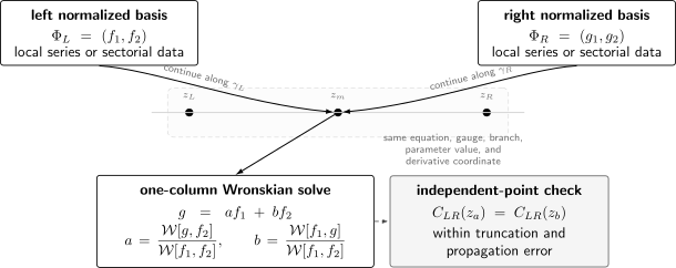
Two normalized endpoint bases are continued along declared paths to one ordinary overlap. Exact jets give the same $C_{LR}$ at every match point; drift when the match point moves diagnoses evaluation error, not new connection data.

The Chapter 2 convention also implies $a_L=C_{LR}a_R$ for the coefficient columns of one fixed solution. Record that direction in a computational manifest: frame transitions and coordinate maps run oppositely.

Abel normalization explains match-point invariance

Abel’s identity gives

$$\frac{\dd}{\dd z}\Wr[u,v] = -p(z)\Wr[u,v].$$

Fix a base point, continuation path, and branch of the integral, and define

$$\mu(z) = \exp\left( \int_{z_*}^{z}p(\zeta)\,\dd\zeta \right).$$

Then the Abel-normalized Wronskian

$$\mathcal W[u,v] = \mu(z)\Wr[u,v](z)$$

is constant on that lifted domain. Every numerator and denominator in a connection coefficient acquires the same Abel factor, so their ratio is constant even when the raw Wronskians are not.

For the nonmonic equation

$$a_2(z)y''+a_1(z)y'+a_0(z)y=0,$$

use $p=a_1/a_2$. In self-adjoint form,

$$\bigl(r(z)y'(z)\bigr)'+s(z)y(z)=0,$$

the constant bilinear object is simply

$$r(z)\Wr[u,v](z).$$

Three statements that are often blurred together should be kept separate:

Statement	Status
$\Wr[u,v]$ is constant	True only when $p=0$ in the chosen gauge
$\mathcal W[u,v]$ is constant	Exact on a fixed lifted path and branch
A computed Wronskian ratio is match-point independent	A numerical claim requiring validation

Four layers of a direct computation

A formula can be exact while its evaluation is unstable. A useful audit therefore assigns a status to each layer rather than labeling the whole calculation “exact” or “numerical.”

Layer	Object	What must be recorded
Global datum	$C_{LR}$ for normalized, path-labelled bases	Basis order, normalization, branches, path, sectors
Algebraic identity	$C_{LR}=J_L^{-1}J_R$ and its Wronskian ratios	Exact, provided both jets solve the same equation
Solution representation	Frobenius series, convergent expansion, asymptotic series, or propagated IVP	Domain of convergence or asymptotic remainder status
Reported value	Finite-precision coefficient or spectral zero	Precision, truncation, solver, conditioning, and independent checks

The following vocabulary will be used throughout the chapter.

• Exact means an identity in the declared equation and normalization.
• Convergent means a representation with a proved or stated convergence domain.
• Asymptotic means a sectorial approximation with an order and remainder interpretation.
• Computed means a finite algorithm has returned a value.
• Validated means independent changes of match point, precision, representation, or propagation direction support the claimed digits.

A truncated divergent expansion does not become exact because it is inserted into an exact Wronskian identity. Conversely, numerical quadrature does not make the underlying connection coefficient a numerical rather than mathematical object.

Every jet must use the same coordinate and gauge

Local bases are often expressed in different variables or gauges. Suppose

$$y(z)=\chi(z)u\bigl(\zeta(z)\bigr).$$

The corresponding jets satisfy

$$\begin{pmatrix} y\\ y_z \end{pmatrix} = \begin{pmatrix} \chi&0\\ \chi'&\chi\zeta' \end{pmatrix} \begin{pmatrix} u\\ u_\zeta \end{pmatrix}.$$

Consequently,

$$\Wr_z[y_1,y_2] = \chi(z)^2\zeta'(z) \Wr_\zeta[u_1,u_2].$$

The factor cancels from a Wronskian ratio only when the same transformation has been applied to every solution in that ratio. Combining a $z$-derivative on one side with a $\zeta$-derivative on the other silently changes the answer.

This rule is especially important after normal-form transformations. A half-density gauge may make the transformed Wronskian constant, but it also changes endpoint amplitudes. The connection matrix in the original physical normalization is recovered only after the full jet transformation is undone.

Keep a scaling ledger

Numerical propagation often rescales columns to avoid overflow or underflow. Let

$$f_j=s_j\widehat f_j, \qquad g=t\widehat g,$$

and suppose

$$\widehat g = \widehat A\widehat f_1 +\widehat B\widehat f_2.$$

Then the coefficients in the original normalization are

$$A=\frac{t}{s_1}\widehat A, \qquad B=\frac{t}{s_2}\widehat B.$$

For full frames, if

$$\Phi_L=\widehat\Phi_LD_L, \qquad \Phi_R=\widehat\Phi_RD_R,$$

and

$$\widehat\Phi_R = \widehat\Phi_L\widehat C_{LR},$$

then

$$C_{LR} = D_L^{-1}\widehat C_{LR}D_R.$$

Rescaling is harmless and often essential. Forgetting the diagonal ledger is not. If propagation uses orthogonalization or another nondiagonal basis change, record the full transformation matrix rather than only its diagonal.

Exact benchmark: a modified-Bessel connection

An exact test should exercise the same sign, Abel, resonance, and scaling logic as a difficult computation. Modified Bessel’s equation,

$$y'' +\frac1z y' -\left( 1+\frac{\nu^2}{z^2} \right)y =0,$$

has $p=1/z$, so $z\Wr$ is constant. Restrict first to positive real $z$, where $I_\nu$ and $K_\nu$ have their standard real normalizations, and take $\nu\notin\mathbb Z$. Then

$$I_{-\nu}(z) = I_\nu(z) +\frac{2\sin(\pi\nu)}{\pi}K_\nu(z),$$

while

$$\Wr[I_\nu,K_\nu] = -\frac1z.$$

Take

$$\Phi_L=(I_\nu,K_\nu), \qquad g=I_{-\nu}.$$

The Wronskian solve gives

$$\frac{\Wr[g,K_\nu]}{\Wr[I_\nu,K_\nu]}=1,$$

and

$$\frac{\Wr[I_\nu,g]}{\Wr[I_\nu,K_\nu]} = \frac{2\sin(\pi\nu)}{\pi}.$$

At $\nu=1/3$, the second coefficient is

$$\frac{\sqrt3}{\pi} \approx 0.551328895421792.$$

This benchmark catches four implementation errors at once:

1. omitting derivatives gives no way to separate the two coefficients;
2. reversing the second Wronskian changes its sign;
3. assuming the raw Wronskian is constant misses its $z^{-1}$ behavior;
4. mixing scaled and unscaled $K_\nu$ values corrupts the amplitude.

At integer $\nu=n$, the pair $(I_\nu,I_{-\nu})$ collapses because $I_{-n}=I_n$. The standard $K_n$ is obtained by a limiting recombination. The apparent singularity of the generic basis formula is therefore a basis artifact, not a singularity of the differential equation. This is the model for handling resonant Frobenius bases throughout the book.

A two-point numerical audit

The exact answer also makes a useful finite-precision unit test. At $\nu=1/3$, evaluate the derivatives independently from

$$\begin{aligned} I_\nu' &= \frac12 \left( I_{\nu-1}+I_{\nu+1} \right), \\ K_\nu' &= -\frac12 \left( K_{\nu-1}+K_{\nu+1} \right). \end{aligned}$$

Using Python 3, mpmath 1.3.0, and mp.dps = 80, with the order recurrences above rather than numerical differentiation, gives:

| Point | Recovered $A$ | Recovered $B$ | $|z\Wr[I_\nu,K_\nu]+1|$ | |---|---:|---:|---:| | $z=0.7$ | $1.000000000000000$ | $0.551328895421792$ | $<10^{-79}$ | | $z=2.3$ | $1.000000000000000$ | $0.551328895421792$ | $<10^{-79}$ |

For $v_h=(h,h')^{\mathsf T}$, define the one-column infinity-norm residual

$$\rho_g = \frac{ \lVert v_g-A v_{I_\nu}-B v_{K_\nu}\rVert_\infty }{ \lVert v_g\rVert_\infty +|A|\lVert v_{I_\nu}\rVert_\infty +|B|\lVert v_{K_\nu}\rVert_\infty }.$$

Using the coefficients solved at $z=0.7$ gives $\rho_g(2.3)<10^{-80}$. The two points differ substantially in the relative sizes of $I_\nu$ and $K_\nu$, so agreement tests more than textual substitution into the connection formula. The printed 15 digits are stable; defects at the working-precision roundoff scale are reported only as order-of-magnitude bounds, not as universal accuracy guarantees.

From local data to a stable match

The Wronskian formula accepts any exact fundamental pair, but a computation must first construct that pair. The appropriate initialization depends on the endpoint.

Endpoint	Initialization	Required ledger
Ordinary	Taylor series or IVP jet	Radius or local error
Regular, nonresonant	Unit-leading Frobenius pair	Power branches and excluded collisions
Regular, resonant	Logarithmic or divided-difference pair	Limit convention and logarithmic coefficient
Irregular	Asymptotic initial data for sectorial solutions	Exact normalization, sector, lateral side, truncation, remainder status

A formal asymptotic series at an irregular endpoint is not itself an exact solution. It supplies approximate initial data at a finite point, and the initialization error must be propagated into the reported coefficient.

Direction matters for recessive solutions

Suppose the desired endpoint solution is recessive while a second solution is dominant. A tiny dominant contamination introduced by roundoff or truncation can overwhelm the desired column when integration proceeds in the direction where the contaminant grows faster. The exact initial-value problem remains well posed, but the chosen numerical representation is unstable.

A practical rule is to continue each endpoint basis toward the overlap in a direction along which the wanted solution grows at least as rapidly as its competitor. If that is impossible for both columns at once, use rescaling, orthogonalization, Riccati variables, exterior products, or a recurrence adapted to the minimal solution. The later pages develop these alternatives.

Match where the frame is well separated

Choose a reference length $\ell>0$ in the numerical coordinate and let

$$v_j^{(\ell)} = \begin{pmatrix} f_j\\ \ell f_j' \end{pmatrix}.$$

The dimensionless scaled area

$$\sigma_F^{(\ell)} = \frac{ \ell\left|\Wr[f_1,f_2]\right| }{ \lVert v_1^{(\ell)}\rVert_2 \lVert v_2^{(\ell)}\rVert_2 }$$

satisfies $0<\sigma_F^{(\ell)}\leq1$ for a fundamental frame. It is invariant under nonzero rescaling of either column. A very small value means the computed columns are nearly parallel relative to their magnitudes, so extracting coordinates will amplify error.

This diagnostic depends on the relative scaling of the value and derivative rows; a change of independent variable can change it. It is a conditioning indicator in a declared numerical coordinate, not a geometric invariant.

For a normwise perturbation analysis, write

$$\begin{aligned} G&=FC,\\ \widehat F&=F+\Delta F,\\ \widehat G&=G+\Delta G. \end{aligned}$$

If

$$\eta=\lVert F^{-1}\Delta F\rVert<1,$$

then

$$\begin{aligned} \widehat C-C &= \left( I+F^{-1}\Delta F \right)^{-1}\\ &\quad{}\times F^{-1} \left( \Delta G-\Delta F\,C \right), \end{aligned}$$

and therefore

$$\lVert\widehat C-C\rVert \leq \frac{\lVert F^{-1}\rVert}{1-\eta} \left( \lVert\Delta G\rVert +\lVert\Delta F\rVert\lVert C\rVert \right).$$

No algebraic rearrangement can remove the factor $\lVert F^{-1}\rVert$. One must improve the frame, the scaling, the match point, the precision, or the representation.

What is deferred to the verification page

The bound above and the second-point test below are the minimum admission checks for every calculation in this chapter. The closing page will go further: a posteriori error budgets, adaptive precision, interval or ball arithmetic, certified root counts, and comparison of independent implementations.

The independent-point test is not optional

At the point used to solve $C=F^{-1}G$, the reconstruction residual $G-FC$ is nearly zero by construction. It is not an independent validation. Continue or reevaluate the same normalized frames at a second point $z_b$ and compute

$$R_b=J_R(z_b)-J_L(z_b)\widehat C.$$

A scale-aware residual is

$$\rho_b = \frac{ \lVert R_b\rVert }{ \lVert J_R(z_b)\rVert +\lVert J_L(z_b)\rVert\lVert\widehat C\rVert }.$$

Now move the matching point through an overlap interval. A plateau of stable digits under changes of point, precision, truncation order, and propagation direction is strong evidence that evaluation error is controlled. It is not evidence that the declared path or branch was the intended one; those are separate semantic checks.

The determinant identity supplies another independent test:

$$\det\widehat C \stackrel{?}{=} \frac{ \mathcal W[g_1,g_2] }{ \mathcal W[f_1,f_2] }.$$

When exact normalizations determine the two Abel-normalized Wronskians, the right side can often be computed without performing the full continuation.

A reproducible eight-step protocol

For a scalar two-end connection problem:

1. Freeze conventions. Record the equation, spectral parameter, gauge, independent variable, ordered bases, leading coefficients, cuts, path classes, sectors, and excluded parameter values.
2. Construct endpoint data. Use a convergent local series or a sectorial asymptotic initialization with a declared remainder status.
3. Continue both frames. Bring all four columns to the same simply connected ordinary overlap without changing their normalization ledger.
4. Unify jets. Convert every value and derivative to the same coordinate and gauge.
5. Balance the frames. Rescale columns, nondimensionalize rows, and choose a point where the frames remain numerically independent.
6. Solve, do not invert. Use a pivoted or orthogonal factorization for $J_LC=J_R$; use the Wronskian formulas as sign and determinant audits.
7. Validate elsewhere. Repeat at independent points and with increased precision or a second representation.
8. Report provenance. Publish the normalization ledger, algorithm, truncation and precision, residuals, conditioning indicator, and stable digits together with the result.

For a boundary problem, suppose the admissible left solution is $f_1$ and the admissible right solution is $g_1$. Since

$$g_1=(C_{LR})_{11}f_1+(C_{LR})_{21}f_2,$$

the two boundary lines align precisely when

$$(C_{LR})_{21} = \frac{\Wr[f_1,g_1]}{\Wr[f_1,f_2]} =0.$$

If the denominator remains nonzero, the spectral condition is the numerator zero. Multiplying either admissible solution by an analytic nowhere-zero factor of the spectral parameter, constant in $z$, preserves this zero and its multiplicity. A normalization factor with its own zeros or poles does not.

Logarithmic derivatives reduce dynamic range

Away from zeros, define

$$m_y=\frac{y'}{y}.$$

Then

$$\Wr[u,v] = uv\left(m_v-m_u\right).$$

Thus a boundary-alignment condition can be tested by equality of logarithmic derivatives when both amplitudes are nonzero. This Riccati formulation often reduces overflow from exponential amplitudes, but it loses amplitude information and develops poles at zeros of the solution. It complements, rather than replaces, the full connection calculation.

A first Heun matching experiment

The next page will derive the local expansions used in an actual Heun calculation. Before doing so, it is useful to specify the experiment so that its later output has an unambiguous target. Take the general Heun equation

$$\begin{aligned} y'' &+ \left( \frac{\gamma}{z} +\frac{\delta}{z-1} +\frac{\epsilon}{z-a} \right)y'\\ &+ \frac{\alpha\beta z-q} {z(z-1)(z-a)} y=0, \end{aligned}$$

with

$$\alpha+\beta+1 = \gamma+\delta+\epsilon.$$

One nonresonant real test case is

$$\begin{aligned} a&=2, & \alpha&=\frac13, & \beta&=\frac7{12},\\ \gamma&=\frac12, & \delta&=\frac23, & \epsilon&=\frac34, & q&=\frac25. \end{aligned}$$

Use the straight interval $0<z<1$ with real positive branches. At $z=0$, choose the unit-leading pair with exponents $0$ and $1/2$; at $z=1$, use the unit-leading pair with exponents $0$ and $1/3$, where the second power is $(1-z)^{1/3}$. Evaluate both frames at $z_m=0.4,0.5,0.6$.

The experiment is accepted only when:

• the same normalization ledger is used at all three points;
• the four entries of $C_{01}$ stabilize as series order and precision grow;
• reconstruction at a point not used for the solve agrees to the claimed digits;
• the determinant agrees with the ratio of the two Abel constants; and
• direct propagation from both ends agrees with a second representation.

No numerical table is printed yet because its quality depends on the recurrence, continuation, and error controls developed on the following pages. Stating the acceptance test before seeing the answer prevents an attractive but unverified number from defining its own standard.

First-order systems use determinant minors

For an $n$-component system

$$Y'(z)=A(z)Y(z),$$

two fundamental matrices satisfy

$$\begin{aligned} \Phi_R&=\Phi_LC_{LR},\\ C_{LR}&=\Phi_L^{-1}\Phi_R,\\ C_{LR}'&=0. \end{aligned}$$

Liouville’s formula is

$$\frac{\dd}{\dd z}\det\Phi = \operatorname{tr}A\,\det\Phi.$$

Therefore

$$\exp\left( -\int_{z_*}^{z}\operatorname{tr}A(\zeta)\,\dd\zeta \right) \det\Phi(z)$$

is constant. The scalar companion matrix has trace $-p$, reproducing Abel’s identity.

Cramer’s rule generalizes the scalar Wronskian formulas:

$$(C_{LR})_{ij} = \frac{ \det\left( \phi_{L,1},\ldots, \phi_{R,j}, \ldots, \phi_{L,n} \right) }{ \det\Phi_L },$$

where $\phi_{R,j}$ replaces column $i$ in the numerator. For subspace boundary conditions, the natural quantities are minors or exterior products—Plücker coordinates—not two-function Wronskians. Numerically, one usually evolves orthogonal factorizations or compound variables rather than expanding large determinants.

How the direct-method chapter fits together

This page supplies the extraction identity and audit protocol. The remaining pages construct increasingly powerful representations of the endpoint solutions.

Page	Direct-method task
Connection coefficients as Wronskian ratios	Continue normalized frames, solve once, and validate independently
Frobenius, Jaffé, and Leaver-type expansions	Build local and globally adapted series with explicit domains
Three-term recurrences and dominant/minimal solutions	Identify the recurrence branch selected by a boundary condition
Perron–Kreuser theory, Pincherle’s theorem, and continued fractions	Turn minimality into a computable continued-fraction condition
Large-order recurrence asymptotics and connection amplitudes	Relate coefficient tails to endpoint connection data
Polynomial truncation, Hill determinants, and quasi-exact solvability	Separate exact termination from approximate determinant roots
Green functions, poles, and QNM conditions from recurrences	Convert recurrence data into spectral and resolvent conditions
Verified numerics	Turn these diagnostics into error budgets, certified roots, precision schedules, and independent implementations

Common pitfalls

Matching values without derivatives. One scalar value cannot determine two coefficients. Match a full value–derivative jet, or an equivalent pair of independent linear functionals.

Calling every Wronskian constant. The raw Wronskian obeys Abel’s identity and usually varies. Ratios are constant only for solutions of the same equation, parameter value, gauge, and continued branch.

Combining incompatible jets. A derivative with respect to $\zeta$ is not a derivative with respect to $z$, and a gauged solution is not the original one. Apply the full jet transformation before taking determinants.

Evaluating a series outside its disk. An exact recurrence does not extend the convergence domain of its Frobenius series. Reexpand, analytically continue, or integrate before matching.

Confusing a stable identity with a stable algorithm. A nonzero exact Wronskian can be much smaller than the computed column magnitudes. Monitor scaled separation and solve with a balanced frame.

Checking only the solve point. The residual at that point is nearly tautological. Test reconstruction at a second point and move the match point through an overlap.

Integrating a recessive solution in the unstable direction. Tiny dominant contamination then grows into the reported solution. Reverse the direction, change representation, or propagate a stabilized subspace.

Interpreting every pole as spectral. At resonance, a standard basis or gamma normalization can degenerate while the equation remains regular in its parameter. Recombine the basis before assigning meaning to the pole.

Exercises

1. Orientation and all four Wronskians

Starting from $g_j=c_{1j}f_1+c_{2j}f_2$, derive the four entries of $C_{LR}$ and its determinant. Then show that if $y=\Phi_La_L=\Phi_Ra_R$, one has $a_L=C_{LR}a_R$.

Solution

Taking the Wronskian of $g_j$ with $f_2$ gives

$$\Wr[g_j,f_2] = c_{1j}\Wr[f_1,f_2].$$

Taking the Wronskian of $f_1$ with $g_j$ gives

$$\Wr[f_1,g_j] = c_{2j}\Wr[f_1,f_2].$$

Therefore, for $j=1,2$,

$$\begin{aligned} (C_{LR})_{1j} &= \frac{\Wr[g_j,f_2]}{\Wr[f_1,f_2]}, \\ (C_{LR})_{2j} &= \frac{\Wr[f_1,g_j]}{\Wr[f_1,f_2]}. \end{aligned}$$

Since $J_R=J_LC_{LR}$,

$$\det C_{LR} = \frac{\det J_R}{\det J_L} = \frac{\Wr[g_1,g_2]}{\Wr[f_1,f_2]}.$$

Finally,

$$\Phi_La_L = \Phi_LC_{LR}a_R,$$

and invertibility of $\Phi_L$ gives $a_L=C_{LR}a_R$.

2. Abel’s identity and the second-point residual

Prove Abel’s identity directly. Then show that an exact $C_{LR}$ computed at $z_a$ also reconstructs $J_R$ at every ordinary point $z_b$ on the same continued branch.

Solution

For two solutions $u,v$,

$$\begin{aligned} \Wr[u,v]' &= uv''-u''v\\ &= u(-pv'-qv)\\ &\quad -(-pu'-qu)v\\ &= -p\Wr[u,v]. \end{aligned}$$

Hence $\mu\Wr$ is constant. For the matrix statement, define $C(z)=J_L(z)^{-1}J_R(z)$. Both jet matrices solve the companion system $J'=AJ$, so

$$\begin{aligned} C' &= -J_L^{-1}AJ_LJ_L^{-1}J_R +J_L^{-1}AJ_R\\ &=0. \end{aligned}$$

Thus $C(z_b)=C(z_a)$ and $J_R(z_b)-J_L(z_b)C(z_a)=0$ exactly. A nonzero computed second-point residual measures representation, propagation, or roundoff error.

3. Modified-Bessel benchmark

Use the identity for $I_{-\nu}$ and $\Wr[I_\nu,K_\nu]=-1/z$ to recover both coefficients by Wronskian ratios. Explain what fails at integer $\nu$.

Solution

Let

$$c_\nu=\frac{2\sin(\pi\nu)}{\pi}, \qquad I_{-\nu}=I_\nu+c_\nu K_\nu.$$

Then

$$\Wr[I_{-\nu},K_\nu] = \Wr[I_\nu,K_\nu],$$

so the $I_\nu$ coefficient is $1$. Also,

$$\Wr[I_\nu,I_{-\nu}] = c_\nu\Wr[I_\nu,K_\nu],$$

so the $K_\nu$ coefficient is $c_\nu$. At integer order, $I_{-n}=I_n$, and the displayed source pair is no longer fundamental. One must replace its vanishing divided difference by the finite logarithmic solution $K_n$ through the standard limit.

4. Coordinate and gauge covariance

For $y(z)=\chi(z)u(\zeta(z))$, derive the jet matrix and Wronskian transformation. State precisely when its determinant factor cancels from a connection coefficient.

Solution

The chain rule gives

$$y_z=\chi'u+\chi\zeta'u_\zeta,$$

and therefore

$$\begin{pmatrix} y\\y_z \end{pmatrix} = \begin{pmatrix} \chi&0\\ \chi'&\chi\zeta' \end{pmatrix} \begin{pmatrix} u\\u_\zeta \end{pmatrix}.$$

Taking determinants of two jet columns gives

$$\Wr_z[y_1,y_2] = \chi^2\zeta'\Wr_\zeta[u_1,u_2].$$

The factor cancels only if the numerator and denominator use the same $\chi$, $\zeta$, point, and derivative convention. With different endpoint gauges, first transform both continued frames into one common jet.

5. A perturbation bound for the matching solve

Let $G=FC$ and let both frames be perturbed. Derive the displayed identity and norm bound for $\widehat C-C$.

Solution

From

$$\widehat C =(F+\Delta F)^{-1}(G+\Delta G)$$

and $G=FC$,

$$\begin{aligned} \widehat C-C &= (F+\Delta F)^{-1} \left( \Delta G-\Delta F\,C \right)\\ &= \left( I+F^{-1}\Delta F \right)^{-1}\\ &\quad{}\times F^{-1} \left( \Delta G-\Delta F\,C \right). \end{aligned}$$

When $\eta=\lVert F^{-1}\Delta F\rVert<1$, the Neumann-series bound gives

$$\left\| \left(I+F^{-1}\Delta F\right)^{-1} \right\| \leq \frac1{1-\eta}.$$

Submultiplicativity and the triangle inequality give the stated result.

6. Normalization factors and spectral zeros

Suppose a boundary coefficient is

$$B(\lambda) = \frac{ \Wr[f_1,g] }{ \Wr[f_1,f_2] }.$$

Find its transformation when $f_1=s_1\widehat f_1$, $f_2=s_2\widehat f_2$, and $g=t\widehat g$. Which rescalings preserve the zeros and their multiplicities?

Solution

Both factors in each Wronskian depend only on the parameter, not on $z$, so

$$B(\lambda) = \frac{t(\lambda)}{s_2(\lambda)} \frac{ \Wr[\widehat f_1,\widehat g] }{ \Wr[\widehat f_1,\widehat f_2] } = \frac{t}{s_2}\widehat B.$$

Analytic nowhere-zero $t/s_2$ preserves every zero and its multiplicity. Zeros or poles of the normalization factor can create, remove, or change the apparent multiplicity of spectral zeros. The factor $s_1$ cancels because it occurs in both numerator and denominator.

7. Riccati matching

Assume $u$ and $v$ are nonzero at $z_m$. Prove that $\Wr[u,v](z_m)=0$ exactly when their logarithmic derivatives agree there. Why is this not a complete connection-coefficient method?

Solution

Since $u'=um_u$ and $v'=vm_v$,

$$\Wr[u,v] = uv(m_v-m_u).$$

With $uv\neq0$, the Wronskian vanishes exactly when $m_u=m_v$. This is enough to test alignment of two one-dimensional boundary subspaces. It does not retain their relative amplitudes, cannot recover a full connection matrix by itself, and has poles wherever either solution vanishes.

8. System determinants and replacement columns

For $Y'=AY$, prove Liouville’s formula and the replacement-column expression for $(C_{LR})_{ij}$. Explain why higher-dimensional boundary subspaces require minors rather than ordinary two-function Wronskians.

Solution

Jacobi’s determinant formula gives

$$\begin{aligned} \frac{\dd}{\dd z}\det\Phi &= \det\Phi\, \operatorname{tr}\left(\Phi^{-1}\Phi'\right)\\ &= \operatorname{tr}A\,\det\Phi. \end{aligned}$$

The normalized determinant follows by integration. Each column of $C_{LR}=\Phi_L^{-1}\Phi_R$ solves a linear system with coefficient matrix $\Phi_L$. Cramer’s rule replaces column $i$ of $\Phi_L$ by the corresponding right-frame column $\phi_{R,j}$, giving the stated determinant ratio. For a $k$-dimensional subspace, its coordinates are $k\times k$ minors, or equivalently components of a wedge product in $\bigwedge^k\mathbb C^n$. A two-column Wronskian records only the special scalar second-order case.

References

• NIST Digital Library of Mathematical Functions, §1.13, Differential Equations, especially Abel’s identity and Wronskians.
• NIST Digital Library of Mathematical Functions, §3.7, Ordinary Differential Equations, for numerical propagation and dominant-solution contamination.
• NIST Digital Library of Mathematical Functions, §10.27, Connection Formulas and §10.28, Wronskians and Cross-Products, for the modified-Bessel benchmark.
• NIST Digital Library of Mathematical Functions, §31.18, Methods of Computation, for Frobenius initialization, numerical continuation, value–derivative matching, and stable integration directions for Heun equations.
• F. W. J. Olver, Asymptotics and Special Functions, A K Peters, 1997, DOI: 10.1201/9781439864548.
• A. B. Olde Daalhuis and F. W. J. Olver, “On the Asymptotic and Numerical Solution of Linear Ordinary Differential Equations,” SIAM Review 40 (1998), 463–495, DOI: 10.1137/S0036144597315341.
• Nicholas J. Higham, Accuracy and Stability of Numerical Algorithms, second edition, SIAM, 2002, DOI: 10.1137/1.9780898718027.
• V. Laĭ, “The Two-Point Connection Problem for Differential Equations of the Heun Class,” Theoretical and Mathematical Physics 101 (1994), 1413–1418, DOI: 10.1007/BF01035461.
• W. Lay, K. Bay, and S. Yu. Slavyanov, “Asymptotic and Numeric Study of Eigenvalues of the Double Confluent Heun Equation,” Journal of Physics A 31 (1998), 8521–8531, DOI: 10.1088/0305-4470/31/42/011.