Degenerate Fusion and Braiding as Finite Connection Operations

Fusion changes the channel in which a chiral block is expanded; braiding analytically exchanges insertions along a declared path. Neither operation is generically a finite matrix in a nonrational Virasoro theory. The finite $2\times2$ matrices relevant to a second-order ODE appear because the level-two degenerate field allows only two adjacent intermediate primaries.

This page makes that statement exact. It starts from the generic fusion kernel, restricts to the two degenerate branches, identifies the resulting gamma matrix with the unit-leading hypergeometric connection matrix, and then records the braid phases and normalization changes needed to compare CFT and ODE conventions.

Six related objects, six different jobs

Object	What it determines	Generic form
Fusion rule	Which intermediate modules are allowed	Spectrum or selection statement
Fusion kernel	Change between chiral block channels	Integral transform
Degenerate fusing matrix	Channel change after the two-branch restriction	$2\times2$ matrix
Braiding operation	Analytic exchange of insertions	Path-dependent linear map
ODE connection matrix	Change between normalized local solution frames	Constant matrix
Crossing equation	Equality of full correlator decompositions	Includes the spectrum and its discrete sum or continuous integration measure, structure constants, and antiholomorphic pairing

A fusion rule is not a fusing matrix, and a chiral fusing matrix is not by itself a full crossing equation.

A channel is a basis choice

The two local pairings

$$\left[ V_{-b/2}(z)V_{\alpha_0}(0) \right]_{\alpha_0^{[\epsilon_0]}} \qquad\longleftrightarrow\qquad \left[ V_{\alpha_1}(1)V_{-b/2}(z) \right]_{\alpha_1^{[\epsilon_1]}}$$

indicate which degenerate OPE is resolved first. The primary at infinity, together with the unpaired finite primary, completes the four-point block. In the first channel the degenerate field approaches $V_{\alpha_0}$; in the second it approaches $V_{\alpha_1}$. The intermediate primary label indexes a basis of chiral blocks. The descendant sums have already been resummed inside each block, so a change of channel acts on primary labels rather than on individual descendants.

For four generic nondegenerate Virasoro representations, a channel change has the schematic form

$$\mathcal V_{\alpha_s}^{(s)}(z) = \int_{\mathcal C} \dd\mu(\alpha_t)\, \mathsf F_{\alpha_s\alpha_t}\, \mathcal V_{\alpha_t}^{(t)}(1-z).$$

The contour $\mathcal C$, the placement of the measure, and the normalization of the kernel $\mathsf F$ depend on the analytic and CFT conventions. In unitary Liouville theory one may parameterize the continuous spectrum by

$$\alpha_t = \frac{Q_{\mathrm L}}2+\ii P_t, \qquad P_t\in\mathbb R_{\ge0}.$$

Here $P_t\leftrightarrow-P_t$ is the Liouville reflection. The integration is over primary representation labels. Every integrand block still contains its complete descendant tower.

The Ponsot–Teschner fusion kernel is therefore an infinite-dimensional integral operator. Rational CFTs instead have finitely many simple modules and finite fusion rules. The particular two-dimensional reduction here comes from inserting the $(2,1)$ degenerate module.

The null relation leaves two primary channels

The previous pages established the fusion rule

$$V_{-b/2}\times V_{\alpha_i} \longrightarrow V_{\alpha_i-b/2} \oplus V_{\alpha_i+b/2}.$$

Instantiate the earlier fusion sign at the collision point $i$ by

$$\alpha_i^{[\epsilon_i]} = \alpha_i-\epsilon_i\frac b2, \qquad \epsilon_i=\pm1.$$

Thus $\epsilon_i=+1$ labels the minus momentum shift. The raw BPZ power is

$$\rho_{i,\epsilon_i} = \frac{bQ_{\mathrm L}}2 + \epsilon_i b\,a_{\mathrm L,i}.$$

The complete branch ledger is:

Collision	Sign	Intermediate momentum	Raw local power
$z\to0$	$+$	$\alpha_0-b/2$	$z^{\rho_{0,+}}$
$z\to0$	$-$	$\alpha_0+b/2$	$z^{\rho_{0,-}}$
$z\to1$	$+$	$\alpha_1-b/2$	$(1-z)^{\rho_{1,+}}$
$z\to1$	$-$	$\alpha_1+b/2$	$(1-z)^{\rho_{1,-}}$

Only the number of allowed intermediate primaries has become finite. Each internal module is generically infinite-dimensional, and each chiral block remains an infinite descendant series.

Ordered unit-leading BPZ frames

On the cut plane used in Chapter 2, take $\Log z$ and $\Log(1-z)$ real for $0<z<1$. Recall the scalar gauge from the BPZ reduction

$$S(z) = z^{\rho_{0,+}} (1-z)^{\rho_{1,+}}.$$

Let $(f_0,g_0)$ and $(f_1,g_1)$ be the unit-leading Gauss bases at zero and one, with the $(A,B,C)$ parameters from that reduction. Define the ordered row frames

$$\begin{aligned} \boldsymbol{\mathscr B}_0 &= \left( \mathscr B_{0,+}, \mathscr B_{0,-} \right) = S(z) \left( f_0,g_0 \right), \\ \boldsymbol{\mathscr B}_1 &= \left( \mathscr B_{1,+}, \mathscr B_{1,-} \right) = S(z) \left( f_1,g_1 \right). \end{aligned}$$

The shared scalar gauge has unit leading coefficient at both endpoints on $0<z<1$. Consequently, these are simultaneously unit-leading BPZ block representatives and unit-leading Frobenius columns: after extracting the displayed local power, the remaining coefficient is one.

The degenerate channel change is the Gauss gamma matrix

Work on

$$\Omega_{01} = \mathbb C \setminus \left( (-\infty,0]\cup[1,\infty) \right),$$

with base point $z_*=1/2$. Declare the matrix direction before writing any coefficient:

$$\boldsymbol{\mathscr B}_0 = \boldsymbol{\mathscr B}_1 C_{10}^{\mathrm{BPZ}}.$$

Equivalently,

$$\mathscr B_{0,\epsilon_0} = \sum_{\epsilon_1=\pm1} \mathscr B_{1,\epsilon_1} \left( C_{10}^{\mathrm{BPZ}} \right)_{\epsilon_1,\epsilon_0}.$$

Rows of $C_{10}^{\mathrm{BPZ}}$ are ordered by $\epsilon_1=(+,-)$; columns are ordered by $\epsilon_0=(+,-)$. To keep the gamma arguments readable, set

$$\Xi_{\epsilon_1,\epsilon_0}^{\pm} := \frac12 + \epsilon_0b\,a_{\mathrm L,0} - \epsilon_1b\,a_{\mathrm L,1} \pm b\,a_{\mathrm L,\infty}.$$

Then the exact finite-$b$ matrix is

$$\left( C_{10}^{\mathrm{BPZ}} \right)_{\epsilon_1,\epsilon_0} = \frac{ \Gamma\!\left( -2\epsilon_1b\,a_{\mathrm L,1} \right) \Gamma\!\left( 1+2\epsilon_0b\,a_{\mathrm L,0} \right) }{ \Gamma\!\left( \Xi_{\epsilon_1,\epsilon_0}^{+} \right) \Gamma\!\left( \Xi_{\epsilon_1,\epsilon_0}^{-} \right) }.$$

No new continuation theorem is being used here. Substituting

$$\begin{aligned} A &= \frac12 +b \left( a_{\mathrm L,0} +a_{\mathrm L,1} -a_{\mathrm L,\infty} \right), \\ B &= \frac12 +b \left( a_{\mathrm L,0} +a_{\mathrm L,1} +a_{\mathrm L,\infty} \right), \\ C &= 1+2b\,a_{\mathrm L,0} \end{aligned}$$

into the Chapter 2 gamma matrix gives this expression entry by entry. A useful generic, nonresonant audit is

$$\det C_{10}^{\mathrm{BPZ}} = -\frac{a_{\mathrm L,0}}{a_{\mathrm L,1}}.$$

This determinant checks the basis order and matrix direction. It is not a normalization-independent observable.

The scalar-coefficient convention is transposed

Many CFT references write each scalar expansion as

$$\mathscr B_{0,\epsilon_0} = \sum_{\epsilon_1=\pm1} \mathsf M_{\epsilon_0,\epsilon_1} \mathscr B_{1,\epsilon_1}.$$

Comparison with the right-multiplying row-frame convention gives

$$\mathsf M_{\epsilon_0,\epsilon_1} = \left( C_{10}^{\mathrm{BPZ}} \right)_{\epsilon_1,\epsilon_0}, \qquad \mathsf M = \left( C_{10}^{\mathrm{BPZ}} \right)^{\mathsf T}.$$

This transpose is bookkeeping, not new physics. It is nevertheless one of the most common sources of an incorrect connection formula.

Braiding is diagonal only in its local channel

Choose a local collision coordinate

$$x_0=z, \qquad x_1=1-z.$$

A signed half-turn is

$$x_i \longmapsto \ee^{\sigma\pi\ii}x_i, \qquad \sigma=\pm1.$$

Because $\mathscr B_{i,\epsilon_i}\sim x_i^{\rho_{i,\epsilon_i}}$, the local phase matrix is

$$\mathsf R_i^{(\sigma)} = \operatorname{diag} \left( \ee^{\sigma\pi\ii\rho_{i,+}}, \ee^{\sigma\pi\ii\rho_{i,-}} \right).$$

Equivalently, each diagonal entry is the branchwise chiral phase

$$\begin{aligned} \left( \mathsf R_i^{(\sigma)} \right)_{\epsilon_i,\epsilon_i} &= \ee^{\sigma\pi\ii\rho_{i,\epsilon_i}} \\ &= \exp \Biggl\{ \sigma\pi\ii \Biggl[ \Delta^{\mathrm{CFT}} \left( \alpha_i^{[\epsilon_i]} \right) - \Delta^{\mathrm{CFT}} \left( -\frac b2 \right) - \Delta_i^{\mathrm{CFT}} \Biggr] \Biggr\}. \end{aligned}$$

A half-turn exchanges endpoint orderings. Calling $\mathsf R_i^{(\sigma)}$ a braid endomorphism therefore also requires an identification of the two ordered block spaces, a tangential coordinate, and any conformal Jacobian convention. A closed positive loop is unambiguous:

$$D_i = \operatorname{diag} \left( \ee^{2\pi\ii\rho_{i,+}}, \ee^{2\pi\ii\rho_{i,-}} \right).$$

In the zero-adapted frame,

$$M_0^{(0)} = D_0, \qquad M_1^{(0)} = \left( C_{10}^{\mathrm{BPZ}} \right)^{-1} D_1 C_{10}^{\mathrm{BPZ}}.$$

Conversely, the loop about zero expressed in the one-adapted frame is

$$M_0^{(1)} = C_{10}^{\mathrm{BPZ}} D_0 \left( C_{10}^{\mathrm{BPZ}} \right)^{-1}.$$

Fusion changes the local basis; conjugation transports the diagonal local monodromy into that new basis.

A lateral path supplies an extra phase ledger

The zero-to-one connection inside $\Omega_{01}$ carries no upper/lower label. If a basis to the right of $1$ is instead normalized with $(z-1)^\rho$, let $\gamma_s$ pass through the upper half-plane for $s=+1$ and the lower half-plane for $s=-1$. Then

$$\left. (1-z)^\rho \right|_{\gamma_s} = \ee^{-s\pi\ii\rho} (z-1)^\rho.$$

Thus the right-normalized frame introduces

$$P_1^{(s)} = \operatorname{diag} \left( \ee^{-s\pi\ii\rho_{1,+}}, \ee^{-s\pi\ii\rho_{1,-}} \right).$$

The sign belongs to the declared local coordinate and path. It should never be guessed from a diagram alone.

Normalization decides which finite matrix is quoted

The matrix above belongs to unit-leading blocks. Chiral vertex operators, reflection conventions, or absorbed OPE factors can rescale the two columns independently. Let

$$N_i = \operatorname{diag} \left( n_{i,+}, n_{i,-} \right), \qquad \widetilde{\boldsymbol{\mathscr B}}_i = \boldsymbol{\mathscr B}_iN_i.$$

The rescaled connection relation is

$$\widetilde{\boldsymbol{\mathscr B}}_0 = \widetilde{\boldsymbol{\mathscr B}}_1 \widetilde C_{10}.$$

When the tilded frames use the chosen chiral-vertex normalization, their finite degenerate fusing matrix is

$$\mathsf F_{10}^{\mathrm{deg}} := \widetilde C_{10} = N_1^{-1} C_{10}^{\mathrm{BPZ}} N_0.$$

This naming does not remove its dependence on $N_0$ and $N_1$.

This covariance is the bridge between an ODE connection matrix and a degenerate CFT fusing matrix.

Layer	Basis normalization	Channel-change object
Gauss functions	Unit-leading $f_i,g_i$	Chapter 2 $C_{10}$
Raw BPZ blocks	Shared scalar gauge times unit-leading bases	$C_{10}^{\mathrm{BPZ}}=C_{10}$
Chiral vertex blocks	Convention-dependent diagonal $N_i$	$N_1^{-1}C_{10}^{\mathrm{BPZ}}N_0$
Full correlator	Adds the spectrum and its discrete sum or continuous integration measure, structure constants, antiholomorphic blocks, and their pairing	Crossing equation

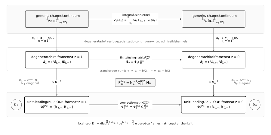
The generic fusion kernel becomes a two-channel operation only after the degenerate pole–residue specialization. The precise normalization relation is $\mathsf F_{10}^{\mathrm{deg}} =N_1^{-1}C_{10}^{\mathrm{BPZ}}N_0$. The two matrices coincide in the unit-leading convention $N_0=N_1=I$.

Changing a local coordinate also illustrates the direction of this rescaling. An unchanged unit-leading solution $\mathscr B_{i,\epsilon_i}\sim x_i^{\rho_{i,\epsilon_i}}$ has leading coefficient $\lambda_i^{-\rho_{i,\epsilon_i}}$ when written in $\widetilde x_i=\lambda_i x_i$. Re-normalizing it to be unit-leading in $\widetilde x_i$ means $\widetilde{\boldsymbol{\mathscr B}}_i =\boldsymbol{\mathscr B}_iN_i^{(\lambda)}$, with

$$N_i^{(\lambda)} = \operatorname{diag} \left( \lambda_i^{\rho_{i,+}}, \lambda_i^{\rho_{i,-}} \right),$$

with a declared branch of $\Log\lambda_i$. Likewise, reflection $a_{\mathrm L,i}\mapsto-a_{\mathrm L,i}$ swaps the two branch labels and can introduce a reflection-normalization factor.

What this finite matrix does not yet compute

One degenerate line makes the channel operations involving that line finite. Reassociating unrelated generic background channels can still require an integral kernel. In the five-insertion problem the exact finite-$b$ equation also remains a PDE, despite having two local probe branches.

Later Heun connection coefficients additionally require the classical block, accessory normalization, scalar gauges, continuation paths, and, in some formulas, subleading data. The elementary matrix on this page is one controlled ingredient of that assembly.

Common pitfalls

Calling generic Virasoro fusion a matrix. In the nonrational generic sector it is an integral transform over intermediate primary momentum. The $2\times2$ matrix arises only after the degenerate selection rule and its analytic continuation have been imposed.

Confusing finite channels with finite descendant spaces. The degenerate field restricts the adjacent intermediate primary to two possibilities. The corresponding conformal blocks still resum infinitely many descendants.

Equating a fusion rule with a fusing matrix. The rule lists allowed modules. The matrix compares two ordered and normalized bases of blocks.

Transposing the matrix silently. Scalar CFT coefficients commonly place the source-channel sign first. The book right-multiplies row frames, so rows belong to the target basis and columns to the source basis.

Calling braiding and fusion the same operation. Fusion changes the channel basis; braiding analytically exchanges insertions along a path. A full monodromy is a closed loop and is safer to compare across conventions than a half-braid.

Reading gamma poles as divergent solutions. At resonance the generic power basis can become singular. The solution space remains two-dimensional; take a coordinated resonant or logarithmic basis limit before interpreting the matrix.

Exercises

1. Separate channel counting from descendant counting

List the two intermediate momenta in $V_{-b/2}\times V_{\alpha_0}$. Why does the corresponding block space still contain infinite series, and why is the resulting two-channel chiral relation not yet a full crossing equation?

Solution

The two allowed primary momenta are

$$\alpha_0-\frac b2, \qquad \alpha_0+\frac b2.$$

The fusion rule restricts only the intermediate highest weights. Each intermediate module generically has descendants at arbitrarily high level, and the chiral block sums their contributions. The null relation reduces the coordinate dependence to a second-order equation; it does not truncate every descendant tower to finite dimension.

A full crossing equation compares full correlator decompositions. It also requires the spectrum and its discrete sum or continuous integration measure, structure constants, the antiholomorphic blocks, and a pairing that produces the full correlator. The two-channel chiral basis change supplies none of that model-dependent data by itself.

2. Reduce the generic kernel to a two-term transform

Write the channel change after analytically continuing one external momentum to the $(2,1)$ degenerate value.

Solution

For a fixed zero-channel branch $\epsilon_0$, the contour transform reduces to

$$\mathscr B_{0,\epsilon_0} = \sum_{\epsilon_1=\pm1} \mathsf M_{\epsilon_0,\epsilon_1} \mathscr B_{1,\epsilon_1}.$$

In a Liouville-type derivation this is not obtained by naively replacing one momentum in the generic integrand while holding the contour fixed. The degenerate analytic continuation moves or pinches kernel poles; the relevant residues leave the two allowed $z\to1$-channel momenta $\alpha_1-\epsilon_1b/2$.

3. Audit the matrix direction

Convert the scalar relation in Exercise 2 into the book’s row-frame notation.

Solution

The source label $\epsilon_0$ selects a column, while $\epsilon_1$ selects the coefficient of a target-basis element. Therefore

$$\left( C_{10}^{\mathrm{BPZ}} \right)_{\epsilon_1,\epsilon_0} = \mathsf M_{\epsilon_0,\epsilon_1}.$$

With both signs ordered as $(+,-)$,

$$\boldsymbol{\mathscr B}_0 = \boldsymbol{\mathscr B}_1 C_{10}^{\mathrm{BPZ}}, \qquad \mathsf M = \left( C_{10}^{\mathrm{BPZ}} \right)^{\mathsf T}.$$

4. Recover one gamma entry and the determinant

Use the $(A,B,C)$ parameters from the BPZ reduction to derive the $(+,+)$ entry of $C_{10}^{\mathrm{BPZ}}$. Then evaluate its determinant from the Chapter 2 Wronskian identity.

Solution

The analytic-at-zero column expanded into the analytic-at-one column has

$$\left( C_{10}^{\mathrm{BPZ}} \right)_{+,+} = \frac{ \Gamma(C)\Gamma(C-A-B) }{ \Gamma(C-A)\Gamma(C-B) }.$$

Substitution gives

$$\left( C_{10}^{\mathrm{BPZ}} \right)_{+,+} = \frac{ \Gamma\!\left( 1+2b\,a_{\mathrm L,0} \right) \Gamma\!\left( -2b\,a_{\mathrm L,1} \right) }{ \Gamma\!\left( \frac12 +b\,a_{\mathrm L,0} -b\,a_{\mathrm L,1} +b\,a_{\mathrm L,\infty} \right) \Gamma\!\left( \frac12 +b\,a_{\mathrm L,0} -b\,a_{\mathrm L,1} -b\,a_{\mathrm L,\infty} \right) }.$$

The Wronskian result from Chapter 2 is

$$\det C_{10} = \frac{1-C}{A+B-C}.$$

Since $1-C=-2b\,a_{\mathrm L,0}$ and $A+B-C=2b\,a_{\mathrm L,1}$,

$$\det C_{10}^{\mathrm{BPZ}} = -\frac{a_{\mathrm L,0}}{a_{\mathrm L,1}}.$$

5. Rescale both channel frames

Starting from $\widetilde{\boldsymbol{\mathscr B}}_i =\boldsymbol{\mathscr B}_iN_i$, derive the transformed connection matrix.

Solution

Insert $\boldsymbol{\mathscr B}_0 =\boldsymbol{\mathscr B}_1C_{10}^{\mathrm{BPZ}}$:

$$\begin{aligned} \widetilde{\boldsymbol{\mathscr B}}_0 &= \boldsymbol{\mathscr B}_0N_0 \\ &= \boldsymbol{\mathscr B}_1 C_{10}^{\mathrm{BPZ}}N_0 \\ &= \widetilde{\boldsymbol{\mathscr B}}_1 N_1^{-1} C_{10}^{\mathrm{BPZ}}N_0. \end{aligned}$$

Hence

$$\widetilde C_{10} = N_1^{-1} C_{10}^{\mathrm{BPZ}} N_0.$$

Individual entries and the determinant change with these diagonal normalizations; the underlying analytic continuation map does not.

6. Compare a half-braid with a full loop

Compute a positive half-turn and full loop about zero, then express the full loop in the one-adapted frame.

Solution

In the zero-adapted frame,

$$\mathsf R_0^{(+)} = \operatorname{diag} \left( \ee^{\pi\ii\rho_{0,+}}, \ee^{\pi\ii\rho_{0,-}} \right),$$

and

$$D_0 = \left( \mathsf R_0^{(+)} \right)^2 = \operatorname{diag} \left( \ee^{2\pi\ii\rho_{0,+}}, \ee^{2\pi\ii\rho_{0,-}} \right).$$

Since $\boldsymbol{\mathscr B}_0 =\boldsymbol{\mathscr B}_1C_{10}^{\mathrm{BPZ}}$, the same closed loop in the one-adapted frame is

$$M_0^{(1)} = C_{10}^{\mathrm{BPZ}} D_0 \left( C_{10}^{\mathrm{BPZ}} \right)^{-1}.$$

The half-turn additionally changes endpoint ordering, so identifying its matrix before and after the exchange requires a declared braiding convention.

7. Diagnose a resonant gamma matrix

Let $2b\,a_{\mathrm L,0}$ approach an integer. What becomes singular, and what remains well defined?

Solution

The exponent difference at zero is

$$\rho_{0,+}-\rho_{0,-} = 2b\,a_{\mathrm L,0}.$$

At an integer value, the generic diagonal power basis $(\mathscr B_{0,+},\mathscr B_{0,-})$ can fail. Corresponding gamma entries may diverge or vanish because they encode that singular basis choice. The BPZ equation and its two-dimensional solution space remain well defined.

One must construct a resonant Frobenius basis, determining whether a logarithmic term occurs, or take a coordinated parameter limit of both the basis and $C_{10}^{\mathrm{BPZ}}$. A pole of a denominator gamma instead gives a zero through $1/\Gamma$, often signaling a special selection or truncation rather than a divergent solution.

References

• A. A. Belavin, A. M. Polyakov, and A. B. Zamolodchikov, “Infinite Conformal Symmetry in Two-Dimensional Quantum Field Theory”, Nuclear Physics B 241 (1984), 333–380. Degenerate representations, fusion rules, and differential equations.
• S. Ribault, Conformal Field Theory on the Plane, 2014. Virasoro blocks, degenerate fusion, braiding, and normalization conventions.
• B. Ponsot and J. Teschner, “Liouville Bootstrap via Harmonic Analysis on a Noncompact Quantum Group”, 1999. Generic Liouville fusion and braiding as continuous-kernel operations.
• B. Ponsot and J. Teschner, “Clebsch–Gordan and Racah–Wigner Coefficients for a Continuous Series of Representations of $U_q(\mathfrak{sl}(2,\mathbb R))$”, Communications in Mathematical Physics 224 (2001), 613–655. Harmonic-analysis construction underlying the generic fusion kernel.
• J. Teschner, “Liouville Theory Revisited”, Classical and Quantum Gravity 18 (2001), R153–R222. Chiral vertex normalization, braid relations, locality, and bootstrap.
• G. Bonelli, C. Iossa, D. Panea Lichtig, and A. Tanzini, “Irregular Liouville Correlators and Connection Formulae for Heun Functions”, Communications in Mathematical Physics 397 (2023), 635–727. Centered-momentum degenerate blocks and the exact gamma matrix.
• NIST Digital Library of Mathematical Functions, §15.10, Hypergeometric Differential Equation. Unit-leading bases, Wronskians, resonance, and connection formulae.