Stage A: Resurgent Singularities and Stokes Discontinuities

Page 1 constructed a directional Borel–Laplace sum after analytic continuation and growth along one chosen ray. Resurgence asks a more global question: what happens when the Borel germ is continued along many paths, around many singularities, and onto different sheets?

The answer is not merely a list of points. A resurgent singularity comes with a determination, a local singular part, and a rule for how that part reappears after Laplace transformation. In the simplest case a pole contributes one exponential. A logarithmic singularity contributes an exponential times another asymptotic series. Several singularities on one ray are organized by a Stokes automorphism rather than by an unordered sum of residues.

This page develops that analytic language and fixes its signs. It does not yet identify singularities from a spatial Stokes graph, derive an Airy connection matrix, act on Voros symbols, cancel transseries ambiguities, or impose a spectral boundary condition.

Page question

Which continuation data make a Borel germ resurgent, and how do the local singularities determine the signed difference between its two lateral sums?

Status ledger

Statement used on this page	Status
Gevrey-1 gives a convergent Borel germ near the origin	Consequence of the coefficient bound proved on Page 1
Endless continuation beyond the first Borel disk	Additional hypothesis or theorem; not a consequence of Gevrey growth
Exponential growth on diverted infinite rays	Additional summability hypothesis; not part of continuation alone in this book
Pole, logarithm, and algebraic-branch jump formulae	Exact contour calculations under the displayed branch, continuation, growth, and boundary assumptions
Pole-plus-logarithm local form	Definition of the simple-singularity subclass, not a classification of every resurgent singularity
Closure of simple resurgent objects under products	Structural theorem in the appropriate endlessly continuable convolution algebra
Stokes automorphism and its logarithm	Formal identities in a completed action-graded resurgent-symbol algebra
Alien derivative equals a raw first-sheet singular part	True only in an isolated one-singularity calibration; false in general with intervening singularities
Factorial-over-power large order from a dominant algebraic singularity	Darboux consequence under the stated dominance and analyticity hypotheses
Resurgence of normalized WKB solutions	Theorem in the explicitly stated geometric framework; not asserted for every WKB-form ODE
Borel singular values are always a discrete subset of the ordinary plane	False in the intrinsic WKB framework; the singularities are discrete on the Borel surface, while their projections can accumulate
Spatial connection formulae, Voros wall crossing, and exact spectra	Deferred to Pages 3–6

Five analytic levels that should not be collapsed

Let

$$\widehat f(\hbar) = a_0+ \sum_{n\geq1}a_n\hbar^n, \qquad \phi(\xi) := \mathcal B\widehat f(\xi) = \sum_{n\geq1} \frac{a_n}{\Gamma(n)}\xi^{n-1}.$$

The following properties answer different questions.

Level	Required information	What it controls
Gevrey-1	$	a_n
Directional 1-summability	Continuation and exponential growth near one regular ray	One Borel–Laplace sum in that direction
Resurgence	Endless analytic continuation of the Borel germ	Access to isolated singular data on a continuation surface
Summable resurgence near a ray	Resurgence plus exponential-type bounds on the relevant infinite continuations	Ordinary or lateral Laplace sums near that ray
Simple resurgence	Every accessible singular determination has the pole-plus-logarithm form defined below	A stable algebra with singularity extractors and alien calculus

This book uses resurgent for the continuation property. It states the growth hypothesis separately whenever a Laplace integral is needed. Some sources include exponential type in their definition, so the noun alone should never replace a summability passport.

The implications that matter here are therefore

$$\begin{gathered} \text{Gevrey-1} \not\Longrightarrow \text{resurgent}, \qquad \text{resurgent} \not\Longrightarrow \text{summable in every direction}, \\ \text{simple resurgent} \Longrightarrow \text{resurgent}, \qquad \text{resurgent} \not\Longrightarrow \text{simple resurgent}. \end{gathered}$$

Algebraic branch points more general than logarithms, and even more complicated isolated singularities, can occur in resurgent objects. The word simple names a useful closed subclass; it does not mean that every physically interesting Borel singularity is a simple pole.

Endless continuation replaces one disk by a path space

There are two useful levels of the definition.

The fixed-obstacle model

Let $\Omega\subset\mathbb C$ be closed, discrete, and disjoint from a small initial disk about $0$. A germ $\phi\in\mathbb C\{\xi\}$ is $\Omega$-continuable if it admits analytic continuation along every finite path that starts in the initial disk and then stays in $\mathbb C\setminus\Omega$.

This model already forces a change of viewpoint. If two paths $\gamma_1$ and $\gamma_2$ end at the same ordinary point but wind differently around $\Omega$, then

$$\operatorname{cont}_{\gamma_1}\phi \quad\text{and}\quad \operatorname{cont}_{\gamma_2}\phi$$

need not be the same germ. The singular object is more accurately labelled by

$$(\omega,[\gamma]),$$

where $[\gamma]$ is the relevant fixed-endpoint homotopy class. A branch cut is only a drawing used to choose representatives of these classes.

The intrinsic endless version

A convenient plane formulation says that $\phi$ is endlessly continuable if, for every length bound $L>0$, there is a finite set $\Omega_L\subset\mathbb C$ such that $\phi$ can be continued along every path of length less than $L$ that starts at $0$ and avoids $\Omega_L$ after leaving its initial disk. The obstacle set may grow with $L$.

Equivalently, one can work intrinsically with the maximal analytic continuation of the germ: a pointed Riemann surface

$$(\mathcal R,\pi,p_0), \qquad \pi(p_0)=0,$$

on which the continued germ is single-valued. Endless continuation is a controlled path-lifting property of this surface. In the common discrete and log-algebraic models, singularities are isolated on the continuation surface even when their projected values under $\pi$ coincide or accumulate in the ordinary $\xi$-plane.

Discrete upstairs need not mean discrete downstairs

A fixed discrete set $\Omega\subset\mathbb C$ is an excellent first model, but it is not the most general WKB geometry. In the rigorous Borel-surface construction stated later, critical paths form a discrete set on the Borel surface, while their central-charge images in $\mathbb C_\xi$ may have accumulation points.

A Gevrey-1 series is called resurgent on this page when its shifted Borel germ is endlessly continuable. To form a lateral sum one still needs the boundary continuations and exponential bounds from Page 1.

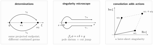
Three pieces of resurgent bookkeeping. Left: paths that end over the same projected value can define different determinations. Center: an accessible singularity carries a pole datum and a cut jump, encoded below as $\mathcal J_\omega\phi=c\delta+g$. Right: convolution can create a singularity at the summed action $\omega_1+\omega_2$, often on a later sheet. The displayed cuts and paths are choices; the continued germs and their monodromy are the analytic data.

A simple singularity carries a pole datum and a minor

Fix a continuation path $\gamma$ from the base germ to a punctured neighborhood of an accessible singularity $\omega$. For the local sign calibration, rotate the singular ray to the positive real axis; a general ray is restored by the inverse orientation-preserving rotation. Put

$$s=\xi-\omega$$

and slit the local $s$-disk along $s>0$. Let $\Log$ denote the principal logarithm, so $\Log(-s)$ has that positive-$s$ cut. We use the following jump-normalized simple form:

$$\begin{aligned} \operatorname{cont}_{\gamma}\phi(\omega+s) ={}& -\frac{c_{\omega,\gamma}}{2\pi\ii\,s} \\ &- \frac{g_{\omega,\gamma}(s)}{2\pi\ii} \Log(-s) +r_{\omega,\gamma}(s), \end{aligned}$$

where $g_{\omega,\gamma}$ and $r_{\omega,\gamma}$ are holomorphic germs at $s=0$. The signs are chosen to agree with Page 1’s convention

$$+=\text{above the positive ray}, \qquad -=\text{below the positive ray}.$$

Indeed, for $s>0$,

$$\Log(-s-\ii0)-\Log(-s+\ii0) = -2\pi\ii.$$

Thus the upper-minus-lower boundary jump of the logarithmic term is exactly $g_{\omega,\gamma}(s)$. The pole is not represented by an ordinary boundary function at $s=0$; its clockwise Hankel contour contributes $c_{\omega,\gamma}$.

Package both pieces as

$$\mathcal J_{\omega,\gamma}\phi := c_{\omega,\gamma}\delta +g_{\omega,\gamma}.$$

Here $\delta$ is the formal unit for Borel convolution:

$$\delta*u=u, \qquad \mathcal L_\theta\delta=1.$$

It is bookkeeping for the constant term under inverse Borel transformation, not an ordinary holomorphic function inserted into the Laplace integral.

The germ $g_{\omega,\gamma}$ is the minor. The coefficient $c_{\omega,\gamma}$ is this book’s jump-normalized pole datum; the ordinary complex residue of the continued Borel function is $-c_{\omega,\gamma}/(2\pi\ii)$. In the standard form below, the coefficient convention gives $\alpha=-c_{\omega,\gamma}$ after the local logarithm and orientation have been matched.

The standard Écalle form is often written

$$\frac{\alpha}{2\pi\ii\,s} + \frac{\Phi(s)}{2\pi\ii}\log s +\text{regular}.$$

Changing the incoming determination, the logarithm, or the orientation changes how $(\alpha,\Phi)$ translates to $(c,g)$. With the local cut and lateral orientation just fixed, the book’s normalization is designed so that $(c,g)$ can be read directly from the analytic jump.

A germ is simple resurgent when it is endlessly continuable and every accessible determination at every singularity has such a simple form. In the simple-resurgent algebra used for alien calculus, the extracted minors are themselves resurgent; this recursive closure is what makes the class useful.

A complete local record

For a calculation, record at least

$$\left( \omega, [\gamma], c_{\omega,\gamma}, g_{\omega,\gamma}, \text{cut orientation}, \text{growth sector} \right).$$

The projected point $\omega$ alone does not determine a Stokes constant or a lateral jump.

One singularity becomes one exponentially weighted companion

Retain Page 1’s analytic convention

$$\operatorname{Disc}^{\mathrm{an}}_\theta := \mathcal S_{\theta+}-\mathcal S_{\theta-}.$$

This is the same discontinuity denoted $\operatorname{Disc}_\theta$ on Page 1. The superscript is added here only to distinguish the analytic map from the formal operators introduced below.

Suppose $\arg\omega=\theta$, the simple singularity above is the only obstruction between the two deformed contours, all connecting pieces vanish, and the continued minor has the exponential bounds required for its Laplace integral. Define the formal companion $\widehat\Phi_{\omega,\gamma}$ by

$$\widehat\Phi_{\omega,\gamma}(\hbar) := c_{\omega,\gamma} + \mathcal B^{-1}g_{\omega,\gamma}.$$

Contour deformation then gives

$$\boxed{ \operatorname{Disc}^{\mathrm{an}}_\theta \widehat f = \ee^{-\omega/\hbar} \mathcal S_\theta \widehat\Phi_{\omega,\gamma} }$$

in the common lateral domain. If the companion ray is itself singular, the appropriate continued lateral sum replaces the unadorned $\mathcal S_\theta$ on the right.

The formula has a simple interpretation:

• the singular location $\omega$ fixes the exponential scale $\ee^{-\omega/\hbar}$;
• the pole datum fixes the leading constant multiplying that exponential;
• the logarithmic minor fixes the entire fluctuation series that accompanies it;
• the path $\gamma$ selects the determination from which those data are extracted.

Exponential smallness holds only where

$$\operatorname{Re} \left( \frac{\omega}{\hbar} \right)>0.$$

Outside that sector the same exponential may be oscillatory or dominant. Calling it “nonperturbatively small” without a phase is therefore incomplete.

Pole calibration

If

$$\phi(\xi) = \frac{r}{\xi-\omega},$$

then

$$c_{\omega}=-2\pi\ii r, \qquad g_{\omega}=0.$$

Hence

$$\operatorname{Disc}^{\mathrm{an}}_\theta \widehat f = -2\pi\ii r\, \ee^{-\omega/\hbar}.$$

For Page 1’s nonalternating Euler series, $\omega=1$ and $r=-1$. The result is

$$\operatorname{Disc}^{\mathrm{an}}_0 \widehat E_+ = 2\pi\ii\ee^{-1/\hbar},$$

so no sign has changed between the two pages.

Logarithmic calibration

For $A>0$, take

$$\phi_{\log}(\xi) = -C\Log\left(1-\frac{\xi}{A}\right),$$

where the germ at the origin is fixed by $\Log 1=0$ and then analytically continued along the specified paths.

Its Taylor expansion at the origin is the Borel transform of

$$\widehat f_{\log}(\hbar) = \sum_{m\geq1} \frac{C\,(m-1)!}{A^m} \hbar^{m+1}.$$

For $\xi=A+s$, the upper-minus-lower boundary values of $\Log(1-\xi/A)$ differ by $-2\pi\ii$. Therefore

$$g_A(s)=2\pi\ii C, \qquad c_A=0,$$

and

$$\operatorname{Disc}^{\mathrm{an}}_0 \widehat f_{\log} = 2\pi\ii C\hbar\, \ee^{-A/\hbar}.$$

Compared with a pole, the logarithm shifts the power multiplying the same action exponential. This is the first glimpse of the singularity–large-order dictionary.

An algebraic branch point gives an exact jump

Reparameterize Page 1’s Exercise 4 by setting $A=\omega^{-1}$. The resulting series $\widehat F_{\omega,\beta}:= \widehat F_{1/\omega,\beta}$ is

$$\widehat F_{\omega,\beta}(\hbar) = \sum_{n=0}^{\infty} \frac{\Gamma(n+\beta)}{\Gamma(\beta)} \omega^{-n}\hbar^{n+1},$$

whose shifted Borel transform is

$$\phi_{\omega,\beta}(\xi) = \left(1-\frac{\xi}{\omega}\right)^{-\beta}.$$

Assume here that

$$\omega>0, \qquad 0<\operatorname{Re}\beta<1, \qquad \hbar>0.$$

The restriction on $\beta$ makes the separate boundary integrals locally integrable at the branch point. Continuing the germ from the origin and using the cut $[\omega,\infty)$ gives, for $s>0$,

$$\begin{aligned} \phi_{\omega,\beta}(\omega+s+\ii0) &= \ee^{\ii\pi\beta} \left(\frac{s}{\omega}\right)^{-\beta}, \\ \phi_{\omega,\beta}(\omega+s-\ii0) &= \ee^{-\ii\pi\beta} \left(\frac{s}{\omega}\right)^{-\beta}. \end{aligned}$$

Their difference is

$$2\ii\sin(\pi\beta) \left(\frac{s}{\omega}\right)^{-\beta}.$$

The common segment from $0$ to $\omega$ cancels between the lateral integrals. Translating the remaining cut integral by $\xi=\omega+s$ yields

$$\begin{aligned} \operatorname{Disc}^{\mathrm{an}}_0 \widehat F_{\omega,\beta} ={}& 2\ii\sin(\pi\beta)\, \omega^\beta\ee^{-\omega/\hbar} \\ &\times \int_0^\infty \ee^{-s/\hbar}s^{-\beta}\,\dd s. \end{aligned}$$

Using the gamma integral and the reflection identity gives the exact closed form

$$\boxed{ \operatorname{Disc}^{\mathrm{an}}_0 \widehat F_{\omega,\beta} = \frac{2\pi\ii\,\omega^\beta}{\Gamma(\beta)} \hbar^{1-\beta} \ee^{-\omega/\hbar} }.$$

The pole case is recovered by analytic continuation to $\beta=1$: the Borel transform then has residue $-\omega$, so its jump is $2\pi\ii\omega\ee^{-\omega/\hbar}$. At $\beta=1$ the boundary-value integrals themselves require the indentation prescription; one should not obtain the limit by treating them as ordinary improper integrals.

For a complex $\omega$, rotate the Borel ray and the local coordinate together. The convergence condition remains the invariant statement $\operatorname{Re}(\omega/\hbar)>0$.

Lateral sums define the formal Stokes automorphism

An analytic discontinuity and a formal Stokes operator live in different categories. Define the book’s formal Stokes automorphism $\mathfrak S_\theta$ operationally by

$$\boxed{ \mathcal S_{\theta+} = \mathcal S_{\theta-} \circ \mathfrak S_\theta }.$$

It follows immediately that

$$\operatorname{Disc}^{\mathrm{an}}_\theta \widehat f = \mathcal S_{\theta-} \left[ (\mathfrak S_\theta-\operatorname{id}) \widehat f \right].$$

Thus the analytic map $\mathcal S_{\theta+}-\mathcal S_{\theta-}$ is not itself the formal automorphism. Nor should one copy a source’s operator named “$\operatorname{Disc}_\theta$” without checking its definition. A common convention sets

$$\operatorname{Disc}^{\mathrm{ref}}_\theta := \operatorname{id}-\mathfrak S_\theta,$$

which has the opposite formal sign:

$$\mathcal S_{\theta+}-\mathcal S_{\theta-} = -\mathcal S_{\theta-} \circ \operatorname{Disc}^{\mathrm{ref}}_\theta.$$

The operational equation in the box is the reliable translation rule.

Alien derivatives are the logarithmic generators

To resolve the Stokes automorphism by action scale, enlarge the formal algebra to include symbols $\ee^{-\omega/\hbar}$. Assume in this subsection that the projected actions on the chosen ray define a locally finite positive grading—or, more generally, a filtration in which every truncation contains only finitely many terms—and complete the algebra in increasing action. In the simple-resurgent setting, define the dotted alien derivations by the homogeneous pieces of

$$\log\mathfrak S_\theta = \sum_{\arg\omega=\theta} \dot\Delta_\omega, \qquad \dot\Delta_\omega := \ee^{-\omega/\hbar}\Delta_\omega.$$

Here $\Delta_\omega$ denotes the generator selected by the chosen lateral continuation prescription at total projected action $\omega$. It is not, in general, a raw extractor attached to one path-labelled local determination. If projected actions accumulate so that the stated filtration is unavailable, this formal exponential needs a more refined topology and is not being asserted by the display.

Equivalently,

$$\mathfrak S_\theta = \exp\left( \sum_{\arg\omega=\theta} \dot\Delta_\omega \right).$$

The sum and exponential are understood grade by grade. The Stokes map is an automorphism,

$$\mathfrak S_\theta(\widehat f\widehat g) = (\mathfrak S_\theta\widehat f) (\mathfrak S_\theta\widehat g),$$

while each homogeneous component of its logarithm is a derivation:

$$\Delta_\omega(\widehat f\widehat g) = (\Delta_\omega\widehat f)\widehat g + \widehat f(\Delta_\omega\widehat g).$$

With $D=\hbar^2\partial_\hbar$, Page 1’s Borel dictionary gives $\mathcal B(D\widehat f)=\xi\mathcal B\widehat f$. The undotted and dotted commutators are

$$\begin{aligned} [D,\Delta_\omega]&=-\omega\Delta_\omega, \qquad [D,\dot\Delta_\omega]&=0. \end{aligned}$$

The factor $\ee^{-\omega/\hbar}$ cancels the first commutator. Thus the undotted $\Delta_\omega$ remembers the action grading, while the dotted operator commutes with $D$ and includes the flat exponential that appears in an analytic jump.

The raw minor is not always the alien derivative

If $\omega$ is the only singularity on the relevant determination, the one-singularity formula calibrates $\Delta_\omega$ directly from the local pair $(c,g)$. With earlier collinear singularities, reaching $\omega$ requires lateral detours, and the logarithm of the full Stokes automorphism contains weighted compositions of those earlier operations. A naive first-sheet minor is then not the alien derivative.

For an action lattice $A,2A,3A,\ldots$, the first two grades illustrate why the logarithm matters:

$$\begin{aligned} \mathfrak S_0\widehat f ={}& \widehat f + \ee^{-A/\hbar}\Delta_A\widehat f \\ &+ \ee^{-2A/\hbar} \left( \Delta_{2A} +\frac12\Delta_A^2 \right)\widehat f +O(\ee^{-3A/\hbar}). \end{aligned}$$

The grade $2A$ contains both primitive data at $2A$ and two successive $A$-operations. Page 7 will turn this action grading into a transseries and study ambiguity cancellation.

An infinite pole lattice can sum to one logarithm

The Stirling series is an exact benchmark with infinitely many Borel singularities. On a fixed logarithm branch, as $\hbar\to0$ with $|\arg(1/\hbar)|\leq\pi-\delta$ for some $\delta>0$, it is the correction in

$$\begin{aligned} \log\Gamma(1/\hbar) \sim{}& \left(\frac1\hbar-\frac12\right) \log(1/\hbar) -\frac1\hbar \\ &+\frac12\log(2\pi) +\widehat\mu(\hbar), \end{aligned}$$

where

$$\widehat\mu(\hbar) = \sum_{k\geq1} \frac{B_{2k}}{2k(2k-1)} \hbar^{2k-1}.$$

In the shifted convention,

$$\mathcal B\widehat\mu(\xi) = \frac1{\xi^2} \left[ \frac{\xi}{2}\coth\left(\frac{\xi}{2}\right)-1 \right].$$

It has simple poles at

$$\omega_m=2\pi\ii m, \qquad m\in\mathbb Z\setminus\{0\},$$

with residue $1/(2\pi\ii m)$. Along the positive imaginary ray, assume $\operatorname{Re}(\ii/\hbar)>0$. Then $q=\ee^{-2\pi\ii/\hbar}$ satisfies $|q|<1$, and the pole formula gives

$$\begin{aligned} \operatorname{Disc}^{\mathrm{an}}_{\pi/2} \widehat\mu &= -\sum_{m\geq1} \frac1m \ee^{-2\pi\ii m/\hbar} \\ &= \log\left( 1-\ee^{-2\pi\ii/\hbar} \right), \end{aligned}$$

where the logarithm is the branch defined by $\log(1-q)=-\sum_{m\geq1}q^m/m$ for $|q|<1$.

This example is deliberately global. Local finiteness of the poles is not enough by itself; the sum of Hankel contributions must converge, and the continuation and large-arc terms must remain controlled.

Convolution creates summed action scales

Page 1 showed that multiplication of formal tails becomes Borel convolution. Let

$$p_A(\xi)=\frac1{A-\xi}, \qquad p_B(\xi)=\frac1{B-\xi},$$

with $A,B,A+B\neq0$ and $A\neq B$. Near $\xi=0$, direct partial fractions give

$$\begin{aligned} (p_A*p_B)(\xi) ={}& \int_0^\xi \frac{\dd\eta} {(A-\eta)(B-\xi+\eta)} \\ ={}& \frac{1}{A+B-\xi} \left[ \Log\left(\frac{A}{A-\xi}\right) + \Log\left(\frac{B}{B-\xi}\right) \right]. \end{aligned}$$

Each $\Log$ initially denotes the germ normalized by $\Log 1=0$. The logarithms create singularities at $A$ and $B$. The denominator also permits a singularity at $A+B$. On one determination the numerator may vanish there; after continuation around $A$ or $B$, it can change by $2\pi\ii$ and expose a genuine pole at $A+B$.

This is the analytic mechanism behind action addition:

$$A,\ B \quad\leadsto\quad A+B.$$

It does not imply that every possible integer combination must occur. Symmetry, vanishing Stokes data, or cancellation on a particular sheet can remove an allowed singularity. The safe claim is that convolution propagates singularities through sums on the continuation surface.

Local singularities forecast large order

Suppose the nearest relevant Borel singularity is at $\omega\neq0$ and, in a domain suitable for Darboux analysis,

$$\phi(\xi) \sim C\left(1-\frac{\xi}{\omega}\right)^{-\beta}.$$

Write the formal tail as

$$\widehat f_+(\hbar) = \sum_{n\geq0}c_n\hbar^{n+1}.$$

Expanding the singular model at the origin and undoing the shifted Borel transform gives

$$c_n \sim \frac{C}{\Gamma(\beta)} \frac{\Gamma(n+\beta)}{\omega^n}.$$

An analytic prefactor at $\omega$ supplies the descending $1/n$ corrections. More distant singularities give exponentially smaller terms in $n$, while several singularities with the same modulus must be added before taking a ratio.

For a conjugate pair, with $\beta$ real,

$$\omega=R\ee^{\ii\varphi}, \qquad \overline\omega=R\ee^{-\ii\varphi},$$

with conjugate amplitudes $C$ and $\overline C$, the leading contribution oscillates:

$$c_n \sim \frac{2|C|\Gamma(n+\beta)} {\Gamma(\beta)R^n} \cos\left( \arg C-n\varphi \right).$$

This is a forecast, not yet the full large-order/transseries theorem. It assumes the displayed singularities dominate, that no equal-modulus contribution was omitted, and that cancellations are treated. Page 7 will derive the companion-sector expansion and ambiguity cancellation systematically.

What is rigorously known for WKB solutions

There is no need to replace every WKB resurgence statement by a conjecture, but the theorem must be named with its domain.

A geometric WKB resurgence theorem

Nikolaev’s 2024 preprint proves the following in Theorem 4.1 and Propositions 4.1–4.6. Let $(X,D)$ be a marked compact Riemann surface with a chosen spin structure, and let $P$ be a Schrödinger operator from $\omega_X^{-1/2}$ to $\omega_X^{3/2}(2D)$. In a local coordinate $z$, write

$$\begin{aligned} P_{\mathrm{loc}} &= \hbar^2\partial_z^2-Q(z,\hbar), \\ P\psi=0 &\Longleftrightarrow \hbar^2\partial_z^2\Psi =Q(z,\hbar)\Psi, \\ Q(z,\hbar) &= \sum_{k=0}^{K}Q_k(z)\hbar^k. \end{aligned}$$

The coefficients $Q_k$ are meromorphic with pole divisors bounded by $2D$, and $D$ is taken minimal. Assume:

1. every zero of the classical quadratic differential $\phi_0=Q_0(z)\,\dd z^2$ is simple;
2. a pole of any higher coefficient $Q_k$ is also a pole of $Q_0$ of at least the same order;
3. the basepoint is regular and one lift to the spectral cover is chosen;
4. the normalized local WKB solution is considered uniformly near that basepoint.

Then the shifted Borel transform of the positive-power tail in the normalized formal WKB amplitude converges and admits endless log-algebraic continuation, uniformly near the basepoint. This continuation statement remains true in unstable directions; what fails there is the exponential-type estimate. In Nikolaev’s stronger terminology, which includes that estimate, the formal WKB solution is resurgent in all but the unstable directions.

The Borel singularities are discrete on the intrinsic Borel surface of critical paths, while their projected central-charge values in the ordinary Borel plane can accumulate. The ordinary or lateral sums used in jump calculations require the stable or semistable trajectory hypotheses stated in the component propositions. An explicit jump additionally requires the local singularity data and contour hypotheses developed above.

This theorem is stronger and more geometric than the informal slogan “WKB singularities occur at periods.” It also explains why the following data cannot be dropped:

Required datum	Role in the theorem or its application
Marked curve and pole divisor	Specify the global equation class and punctures
Spin or half-density data	Make the Schrödinger operator and WKB normalization coordinate compatible
Sheet and regular basepoint	Select one normalized formal WKB branch
Critical path on the spectral cover	Identify a singularity on the Borel surface
Central charge of that path	Project the singularity to an action value in $\mathbb C_\xi$
Phase and trajectory stability	Decide whether the corresponding ray is summable and how its lateral limits behave
Uniformity neighborhood	Control the spatially varying Borel transform

The 2023 peer-reviewed existence and uniqueness theorem cited on Page 1 proves powerful exact-WKB summability results in its stated domains. It should not be silently upgraded into the distinct global resurgence theorem above.

Preprint status

The geometric resurgence result is cited as a preprint and labelled as such. For an ODE outside its structural hypotheses—multiple turning points, different pole behavior, or unproved parameter uniformity—this page treats resurgence and the action dictionary as conditional until an applicable theorem is supplied. In an unstable direction, the continuation statement remains available, but summability and jump claims are withheld without additional growth control.

A Borel Stokes ray is not a spatial Stokes curve

The word Stokes now appears in two related geometries. They must be kept separate until Stage B constructs the bridge.

Stage A: Borel analysis	Stage B: WKB geometry
Variable $\xi$	Spatial variable $z$ on the base curve
Singular ray $\arg\xi=\theta$	Trajectory of a phased quadratic differential
Accessible singularity $(\omega,[\gamma])$	Critical path, saddle trajectory, or action cycle after a theorem identifies it
Lateral contour in the Borel surface	Analytic continuation across a spatial Stokes curve or a graph wall
Abstract $\mathfrak S_\theta$	Concrete transformation of normalized solutions or Voros symbols
Flat factor $\ee^{-\omega/\hbar}$	Exponential of a normalized action integral

Some authors interchange the names Stokes and anti-Stokes for spatial curves. This book will define its trajectory convention from the phase of the quadratic differential on Page 3, rather than infer it from terminology.

The remaining handoff is precise:

• Page 3 builds the phased quadratic differential and its Stokes graph.
• Page 4 fixes canonical sectorial bases and derives local connection formulae.
• Page 5 evaluates Stokes automorphisms on normalized Voros symbols and follows them across graph walls.

Reproducible checks

The companion script resurgent-stokes-discontinuity-check.py verifies, without network access:

1. the shifted Borel coefficients of the algebraic-branch family;
2. the signed pole, logarithmic, and algebraic-branch jumps;
3. recovery of $(\omega,\beta)$ from exact coefficient ratios;
4. the convolution identity and its later-sheet $2\pi\ii$ shift;
5. the first two action grades in the exponential of the alien generator;
6. the residues at the first two poles of the Stirling Borel transform.

It prints the Python, SymPy, and mpmath versions and uses explicit runtime checks, so python3 and python3 -O execute the same audit.

Common pitfalls

Gevrey growth is not resurgence. Gevrey-1 controls only the first Borel disk. A lacunary Borel germ can have a natural boundary even though its inverse formal series is Gevrey-1.

Resurgence is not summability in every direction. Endless continuation does not supply exponential growth at infinity. Every Laplace claim still needs the continuation-and-growth passport from Page 1.

A singular value is not a complete singularity. Different paths can reach different determinations over the same value $\omega$. Always retain the base germ, path class, and sheet.

A branch cut is not invariant data. Moving a cut changes a drawing and the boundary-value bookkeeping. It does not remove the branch point or its monodromy.

A residue is not automatically a Stokes constant. The numerical coefficient depends on the Borel convention, lateral orientation, and normalization of the companion formal sector. Translate all three.

The raw discontinuity is not the logarithmic generator. The full Stokes automorphism contains ordered composites. Alien derivatives are the action-graded pieces of its logarithm.

The nearest point need not control large order alone. Conjugate or equal-modulus singularities can interfere, and a leading amplitude can vanish. Add every dominant contribution before fitting ratios.

A Borel ray is not yet a Stokes curve in the spatial plane. The action map, graph phase, endpoint normalization, and applicable theorem belong to Stage B.

Exercises

Exercise 1 · Gevrey-1 without resurgence

Consider the lacunary Borel germ

$$\phi(\xi) = \sum_{k=0}^{\infty}\xi^{2^k}.$$

Find the formal series whose shifted Borel transform is $\phi$. Show that it is Gevrey-1. What prevents the series from being resurgent?

Solution

The coefficient of $\xi^m$ is one when $m=2^k$ and zero otherwise. Since the shifted transform maps

$$\hbar^{m+1} \longmapsto \frac{\xi^m}{m!},$$

the inverse formal series is

$$\widehat f(\hbar) = \sum_{k=0}^{\infty} (2^k)!\,\hbar^{2^k+1}.$$

Its coefficient $a_n$ is either zero or $(n-1)!$, so

$$|a_n| \leq \Gamma(n) \leq \Gamma(n+1).$$

It is Gevrey-1. The exponent sequence satisfies $2^{k+1}/2^k=2>1$. The Hadamard gap theorem therefore makes the unit circle a natural boundary of $\phi$: the germ cannot be analytically continued through any point of $|\xi|=1$. It is not endlessly continuable and hence is not resurgent.

Exercise 2 · Calibrate a nonconstant minor

Suppose a single singularity at $A>0$ has the book-normalized data

$$\mathcal J_A\phi = 2\pi\ii C\,\delta + 2\pi\ii(m_0+m_1s).$$

Assuming the displayed polynomial minor is the whole continued minor along the positive ray, compute the lateral discontinuity.

Solution

The shifted Laplace moments are

$$\int_0^\infty\ee^{-s/\hbar}\,\dd s = \hbar, \qquad \int_0^\infty s\ee^{-s/\hbar}\,\dd s = \hbar^2.$$

The isolated-singularity formula gives

$$\operatorname{Disc}^{\mathrm{an}}_0\widehat f = 2\pi\ii\ee^{-A/\hbar} \left( C+m_0\hbar+m_1\hbar^2 \right).$$

There is no extra factor $1/\hbar$ because this book uses the shifted Borel transform.

Exercise 3 · Find a singularity on another sheet

Assume $A\neq B$. Derive the convolution formula for $p_A*p_B$. Continue once around $A$ while avoiding $B$. Show how a pole at $A+B$ can appear on the new determination.

Solution

The partial-fraction identity

$$\begin{aligned} &\frac1{(A-\eta)(B-\xi+\eta)} \\ &\qquad= \frac1{A+B-\xi} \left[ \frac1{A-\eta} + \frac1{B-\xi+\eta} \right] \end{aligned}$$

integrates from $0$ to $\xi$ to give the displayed formula in the text. On the initial determination, the logarithmic numerator may tend to zero as $\xi\to A+B$, making the apparent pole removable.

Continuation once around $A$ changes

$$\Log\left(\frac{A}{A-\xi}\right) \longmapsto \Log\left(\frac{A}{A-\xi}\right) \pm2\pi\ii,$$

with the sign fixed by the winding orientation. The continued convolution therefore gains

$$\frac{\pm2\pi\ii}{A+B-\xi},$$

which has a genuine simple pole at the summed action. Its existence and residue are determination-dependent.

Exercise 4 · Expand the Stokes automorphism by action

Assume the positive ray contains action grades $A$ and $2A$ and

$$\log\mathfrak S_0 = \ee^{-A/\hbar}\Delta_A + \ee^{-2A/\hbar}\Delta_{2A} +O(\ee^{-3A/\hbar}).$$

Expand $\mathfrak S_0$ through grade $2A$. Why is the result not just the sum of two local jumps?

Solution

Put

$$X = \ee^{-A/\hbar}\Delta_A + \ee^{-2A/\hbar}\Delta_{2A} +O(\ee^{-3A/\hbar}).$$

Since $\exp X=\operatorname{id}+X+X^2/2+\cdots$, only the square of the grade-$A$ term contributes another grade-$2A$ term. Hence

$$\begin{aligned} \mathfrak S_0 ={}& \operatorname{id} +\ee^{-A/\hbar}\Delta_A \\ &+ \ee^{-2A/\hbar} \left( \Delta_{2A} +\frac12\Delta_A^2 \right) +O(\ee^{-3A/\hbar}). \end{aligned}$$

The composite $\Delta_A^2/2$ records two successive continuations at the first action scale. The full ray jump therefore contains ordered history, not only primitive singularities viewed independently.

Exercise 5 · Translate an opposite Stokes convention

The book defines

$$\mathcal S_+ = \mathcal S_- \circ\mathfrak S.$$

A source instead defines $\widetilde{\mathfrak S}$ by

$$\mathcal S_- = \mathcal S_+ \circ\widetilde{\mathfrak S}.$$

Relate the two automorphisms and write the book’s analytic upper-minus-lower discontinuity using $\widetilde{\mathfrak S}$.

Solution

Substitution gives

$$\mathcal S_- = \mathcal S_- \circ\mathfrak S \circ\widetilde{\mathfrak S}.$$

On the resurgent algebra where the lateral summation map separates the relevant formal symbols,

$$\widetilde{\mathfrak S} = \mathfrak S^{-1}.$$

Therefore

$$\begin{aligned} \mathcal S_+-\mathcal S_- &= \mathcal S_+ \circ (\operatorname{id}-\widetilde{\mathfrak S}) \\ &= \mathcal S_- \circ (\mathfrak S-\operatorname{id}). \end{aligned}$$

Both lines express the same analytic discontinuity; the formal operator changes because the defining direction was reversed.

Exercise 6 · Audit a WKB resurgence slogan

Assess the claim:

Every formal WKB period is resurgent, its Borel singularities are its classical periods, and its positive lateral jump is fixed by the nearest turning point.

Solution

The claim omits the equation class, the dependence on $\hbar$, the marked curve and pole divisor, the sheet, basepoint, and path, and the normalization or regularization of the period. It supplies no Gevrey estimate, endless-continuation theorem, exponential-growth bound, or spatial uniformity.

It also confuses a projected action value with a path-labelled singularity on the Borel surface. “Nearest” is ambiguous when several singularities have equal modulus or lie on different sheets. The sign and coefficient of a lateral jump additionally depend on the Borel normalization, the $+$/$-$ convention, the companion-sector normalization, and all collinear singularities on the ray.

For the geometric theorem stated above, one must check the simple-zero and pole-order assumptions, choose a regular lifted basepoint, and exclude or separately treat unstable directions. Only after Page 3 constructs the graph and Page 5 fixes the Voros normalization can a model-specific period/jump formula be asserted.

References

• D. Sauzin, Introduction to 1-Summability and Resurgence (2014), especially Sections 18–22 on continuation and convolution and Sections 25–30 on simple singularities and alien calculus.
• S. Kamimoto and D. Sauzin, “Iterated Convolutions and Endless Riemann Surfaces,” Annali della Scuola Normale Superiore di Pisa 20 (2020), 177–215. Definitions 1.1–1.2 give a rigorous modern formulation of endless continuability.
• E. Delabaere and F. Pham, “Resurgent Methods in Semi-Classical Asymptotics,” Annales de l’Institut Henri Poincaré, Physique théorique 71 (1999), 1–94. Sections 0.2–0.5 separate continuation, growth, lateral summation, other sheets, and Stokes automorphisms before applying them to WKB.
• D. Dorigoni, “An Introduction to Resurgence, Trans-Series and Alien Calculus,” Annals of Physics 409 (2019), 167914, Sections 3–4. The local signs must be translated through the operational Stokes convention displayed on this page.
• I. Aniceto, G. Başar, and R. Schiappa, “A Primer on Resurgent Transseries and Their Asymptotics,” Physics Reports 809 (2019), 1–135, especially Appendix A for Stokes automorphisms, lateral operators, and alien derivatives.
• M. Loday-Richaud and P. Remy, “Resurgence, Stokes Phenomenon and Alien Derivatives for Level-One Linear Differential Systems,” Journal of Differential Equations 250 (2011), 1591–1630. This gives a rigorous bridge among Borel singularities, alien derivatives, and Stokes–Ramis matrices for the stated system class.
• N. Nikolaev, “Geometry and Resurgence of WKB Solutions of Schrödinger Equations,” (2024 preprint), Theorem 4.1 and Propositions 4.1–4.6. These results supply the geometric Borel surface and the qualified WKB resurgence theorem used above.
• N. Nikolaev, “Existence and Uniqueness of Exact WKB Solutions for Second-Order Singularly Perturbed Linear ODEs,” Communications in Mathematical Physics 400 (2023), 463–517. This is the peer-reviewed summability and exact-solution result used on Page 1; it should not be conflated with the later global resurgence theorem.
• K. Iwaki, Les Houches Lectures on Exact WKB Analysis and Painlevé Equations (2025; revised 2026), Section 1.3.1. The Airy calculation shows how a Borel discontinuity becomes a normalized local WKB connection formula, the subject of Page 4.

Page 3 now supplies the missing spatial geometry: the phased quadratic differential, its trajectories, and the Stokes graph that decides which Borel action becomes visible in which chamber.