A Normalization-Complete Connection-Formula Example

A connection formula becomes a gauge/CFT prediction only after its normalization is complete. Mass shifts, the NS path, the degenerate probe, the scalar gauge, the internal lift, the accessory branch, the two endpoint bases, and the continuation path all affect what the four printed matrix entries mean. This page fixes them once and carries one genuinely four-singular example from beginning to end.

The outcome is a concrete standard-Heun equation at $t=1/25$. A level-two classical-block calculation predicts its unit-leading $0$-to-$t$ connection matrix to about five relative decimal places. An independent Frobenius computation confirms all four entries, while Abel’s identity fixes the determinant exactly. Finally, the numerical matrix is run backward to recover the two block derivatives. That last step turns a comparison into a reversible normalization audit.

The universal factorization was derived on the general-Heun connection page. The purpose here is different: combine it with the Chapter 11 mass passport, accessory passport, and cycle firewall so that the same numerical object can be reconstructed in either direction.

The result in one line

On the real interval $0<z<t=1/25$, with powers normalized in $z$ and $t-z$ and with target rows and source columns ordered as $(-,+)$,

$$\boldsymbol H_0 = \boldsymbol H_t C_{t0}, \qquad C_{t0}^{\mathrm{Frob}} \approx \begin{pmatrix} 0.6852083269&0.5321827959 \\ 1.0471097736&-0.6945959089 \end{pmatrix}.$$

The AGT/classical-block prediction through level two differs by at most $1.09\times10^{-5}$ relatively, entry by entry.

Status ledger

Ingredient	Status in this example
Finite-Omega mass and momentum maps	Algebraically exact in the declared AGT representative
Regular AGT block equality	Used coefficientwise as the normalized formal-series correspondence
Degenerate fusion gamma kernel	Exact at generic nonresonant parameters
Heavy–light passage to the displayed oper	Conditional on derivative-compatible semiclassical factorization
Accessory and endpoint derivatives through $t^2$	Formal sewing series truncated consistently at level two
Direct Frobenius connection matrix for the truncated Heun equation	Independent numerical computation
Wronskian determinant	Exact for the declared unit-leading local bases
Error $O(t^3)$	Numerically observed under consistent level-two truncation and expected from the omitted sewing levels
Global continuation throughout the punctured $t$-plane	Not asserted
Boundary spectrum or nonperturbative completion	Not part of this local connection problem

The page therefore tests a formal small-$t$ connection formula against the exact local solutions of the correspondingly truncated ODE. It does not promote a truncated series to a globally single-valued theorem.

The calculation has one row of data in three languages

Use the weakly coupled regular $SU(2)$ theory with four flavors and the $0t$ sewing channel. The independent centered gauge data are

$$\begin{gathered} q_{\mathrm{UV}}=t=\frac1{25}, \qquad \hbar=\epsilon_1=\frac52, \qquad a_{\mathrm C}=\frac34, \\ (M_1,M_2,M_3,M_4) = \left( \frac12,0,\frac56,0 \right). \end{gathered}$$

Here $a_{\mathrm C}$ is the signed Coulomb representative, not the quadratic gauge-invariant coordinate. The centered localization masses are

$$M_i := \mu_i-\frac{\epsilon_\Sigma}{2}, \qquad \epsilon_\Sigma=\epsilon_1+\epsilon_2.$$

They are held fixed along the NS path. The four puncture masses are

$$\begin{aligned} p_\infty &= \frac{M_1-M_2}{2} =\frac14, & p_1 &= \frac{M_1+M_2}{2} =\frac14, \\ p_t &= \frac{M_3+M_4}{2} =\frac5{12}, & p_0 &= \frac{M_3-M_4}{2} =\frac5{12}. \end{aligned}$$

Thus the ODE exponent coordinates measured by the first Omega plane are

$$\theta_f = \frac{2p_f}{\hbar},$$

or

$$\theta_0=\theta_t=\frac13, \qquad \theta_1=\theta_\infty=\frac15.$$

The internal coordinate is

$$\theta_{0t} = \frac{2a_{\mathrm C}}{\hbar} = \frac35.$$

The scalar Heun equation and the symmetric gamma denominators below are invariant under $a_{\mathrm C}\mapsto-a_{\mathrm C}$. The positive representative is retained so that the gauge passport is reversible; it is not determined by the scalar connection matrix.

These five oriented quantities—not their squares—are the data that select the local exponent ordering and the internal Weyl representative.

Gauge datum	CFT or oper datum	Value
$p_0,p_t$	$a_0=\theta_0/2$, $a_t=\theta_t/2$	$1/6,1/6$
$p_1,p_\infty$	$a_1=\theta_1/2$, $a_\infty=\theta_\infty/2$	$1/10,1/10$
$a_{\mathrm C}$	$a=\theta_{0t}/2=a_{\mathrm C}/\hbar$	$3/10$
$q_{\mathrm{UV}}$	four-point cross-ratio $t$	$1/25$
centered mass scheme	unit-leading, Heisenberg-stripped block scheme	fixed below

The equality $t=q_{\mathrm{UV}}$ belongs to this weak-coupling chart. It is not a convention-free identification in another duality frame.

Finite Ω data identify the path, not just its endpoint

Before taking the NS limit, choose the finite representative

$$\epsilon_1=\frac52, \qquad \epsilon_2=\frac25, \qquad \varepsilon_\star=1, \qquad b=\frac25,$$

with

$$\varepsilon_\star^2=\epsilon_1\epsilon_2, \qquad b^2=\frac{\epsilon_2}{\epsilon_1}.$$

Then

$$\epsilon_\Sigma=\frac{29}{10}, \qquad Q_{\mathrm L}=b+b^{-1}=\frac{29}{10}.$$

The printed localization masses are

$$(\mu_1,\mu_2,\mu_3,\mu_4) = \left( \frac{39}{20}, \frac{29}{20}, \frac{137}{60}, \frac{29}{20} \right),$$

and the Liouville momenta are

$$\begin{aligned} \alpha_\infty &= \frac{Q_{\mathrm L}}2 + \frac{p_\infty}{\varepsilon_\star} = \frac{17}{10}, \\ \alpha_1 &= \frac{Q_{\mathrm L}}2 + \frac{p_1}{\varepsilon_\star} = \frac{17}{10}, \\ \alpha_t &= \frac{Q_{\mathrm L}}2 + \frac{p_t}{\varepsilon_\star} = \frac{28}{15}, \\ \alpha_0 &= \frac{Q_{\mathrm L}}2 + \frac{p_0}{\varepsilon_\star} = \frac{28}{15}, \\ \alpha_{0t} &= \frac{Q_{\mathrm L}}2 + \frac{a_{\mathrm C}}{\varepsilon_\star} = \frac{11}{5}. \end{aligned}$$

These are the book’s uncentered Liouville momenta, for which $\Delta=\alpha(Q_{\mathrm L}-\alpha)$. Bonelli et al. instead denote the centered representatives by $\alpha_f^{\mathrm B}$, with $\Delta=Q_{\mathrm L}^2/4-(\alpha_f^{\mathrm B})^2$. Thus

$$\alpha_f^{\mathrm B} = \alpha_f-\frac{Q_{\mathrm L}}2,$$

before their classical variable $a_f=b\alpha_f^{\mathrm B}$ is identified with the book’s $\theta_f/2$.

The NS path is

$$\epsilon_2\longrightarrow0, \qquad \epsilon_1=\hbar, \qquad M_i, a_{\mathrm C}, t\ \text{fixed}.$$

At its endpoint, $\epsilon_\Sigma\to5/2$. The printed masses therefore move to

$$(\mu_1,\mu_2,\mu_3,\mu_4)_{\mathrm{NS}} = \left( \frac74, \frac54, \frac{25}{12}, \frac54 \right),$$

while the centered $M_i$, the $p_f$, and all five $\theta$ coordinates remain fixed.

Do not freeze the printed masses

Holding $\mu_i$ fixed while $\epsilon_2\to0$ changes $M_i=\mu_i-\epsilon_\Sigma/2$. It is a different path through the finite-Omega parameter space. The leading exponent differences can hide this mistake, but subleading mass contacts and normalized coupling derivatives need not agree.

The finite-Omega point performs two jobs. It fixes the square-root and Liouville-reflection representatives used by AGT, and it records which quantities are transported to the classical $b\to0$ endpoint. One cannot reconstruct that path from the endpoint Heun equation alone.

The NS oper becomes one declared Heun equation

Use the standard general-Heun convention

$$\begin{aligned} 0={}&y''(z) + \left( \frac{\gamma_{\mathrm H}}z + \frac{\delta_{\mathrm H}}{z-1} + \frac{\epsilon_{\mathrm H}}{z-t} \right)y'(z) \\ &+ \frac{ \alpha_{\mathrm H}\beta_{\mathrm H}z -\mathfrak q_{\mathrm H} }{ z(z-1)(z-t) }y(z). \end{aligned}$$

The oriented exponent dictionary is

$$\begin{aligned} \gamma_{\mathrm H} &=1-\theta_0, & \delta_{\mathrm H} &=1-\theta_1, & \epsilon_{\mathrm H} &=1-\theta_t, \\ \alpha_{\mathrm H} &= \frac{ 2-\theta_0-\theta_1-\theta_t+\theta_\infty }{2}, & \beta_{\mathrm H} &= \frac{ 2-\theta_0-\theta_1-\theta_t-\theta_\infty }{2}. \end{aligned}$$

For the selected masses this gives

$$\gamma_{\mathrm H} = \epsilon_{\mathrm H} = \frac23, \qquad \delta_{\mathrm H}=\frac45, \qquad \alpha_{\mathrm H}=\frac23, \qquad \beta_{\mathrm H}=\frac7{15}.$$

The Fuchs relation is an immediate check:

$$\alpha_{\mathrm H}+\beta_{\mathrm H}+1 = \gamma_{\mathrm H}+\delta_{\mathrm H} +\epsilon_{\mathrm H} = \frac{32}{15}.$$

To expose how the internal channel fixes the accessory, introduce

$$\delta_j := \frac{1-\theta_j^2}{4}, \qquad \kappa := \delta_{0t}-\delta_0-\delta_t,$$

and

$$\Lambda := \delta_\infty-\delta_0-\delta_t-\delta_1.$$

For this branch,

$$\begin{gathered} \delta_0=\delta_t=\frac29, \qquad \delta_1=\delta_\infty=\frac6{25}, \qquad \delta_{0t}=\frac4{25}, \\ \kappa=-\frac{64}{225}, \qquad \Lambda=-\frac49. \end{gathered}$$

In the unit-leading, Heisenberg-stripped normalization, the exact coordinate conversion from the reduced classical block $\widehat f$ to the standard Heun accessory is

$$\begin{aligned} \mathfrak q_{\mathrm H} ={}& \frac{\gamma_{\mathrm H}}2 \left( t\delta_{\mathrm H}+\epsilon_{\mathrm H} \right) +t\Lambda -(t-1)\kappa \\ &- t(t-1)\partial_t\widehat f. \end{aligned}$$

The internal weight $\delta_{0t}=1/4-a^2=4/25$—equivalently the centered momentum square $a^2=(3/10)^2$—selects the block/accessory branch. The positive lift $a=+3/10$ is retained separately in the connection passport. Through level two,

$$\widehat f(t) = \frac2{25}t + \frac{587}{11700}t^2 +O(t^3).$$

Substitute this jet into the exact accessory relation, re-expand, and discard the incomplete $t^3$ coefficient. The consistently truncated result is

$$\mathfrak q_{\mathrm H}^{[2]}(t) = -\frac{14}{225} +\frac{14}{75}t +\frac{119}{5850}t^2.$$

At $t=1/25$,

$$\mathfrak q_{\mathrm H}^{[2]} = -\frac{200081}{3656250} \approx -0.0547230085470085.$$

Consequently the equation used in the numerical audit is

$$\begin{aligned} 0={}&y'' + \left[ \frac{2}{3z} + \frac{4}{5(z-1)} + \frac{2}{3(z-1/25)} \right]y' \\ &+ \frac{ \dfrac{14}{45}z +\dfrac{200081}{3656250} }{ z(z-1)(z-1/25) }y. \end{aligned}$$

All four regular singularities are genuine: none of the three finite poles cancels. The internal momentum does not introduce another singularity. On the untruncated formal branch it selects the accessory equivalently to the lifted composite monodromy class

$$\operatorname{tr}(M_0M_t) = -2\cos\left(\frac{3\pi}{5}\right) = \frac{\sqrt5-1}{2}.$$

The equation printed above uses the accessory only through $t^2$, so its directly computed finite-$t$ composite trace realizes this target through the retained sewing order rather than as an exact identity.

What the accessory knows

The standard Heun accessory is fixed here by a normalized classical coupling derivative and an affine scalar-gauge conversion. It does not by itself retain the sign of $a_{\mathrm C}$, the endpoint derivatives needed below, or the continuation path. Those are separate rows of the passport.

Unit-leading frames make the four numbers meaningful

Take

$$0<t<1, \qquad 0<z<t,$$

and choose $\Log z$, $\Log(t-z)$, and $\Log(1-t)$ real on this interval. The continuation path $\beta_{0t}$ stays inside the interval and winds around no other puncture.

Order the source and target row frames as

$$\boldsymbol H_0 = (H_{0,-},H_{0,+}), \qquad \boldsymbol H_t = (H_{t,-},H_{t,+}),$$

with unit-leading germs

$$\begin{aligned} H_{0,-}(z) &=1+O(z), & H_{0,+}(z) &=z^{1/3}[1+O(z)], \\ H_{t,-}(z) &=1+O(t-z), & H_{t,+}(z) &=(t-z)^{1/3}[1+O(t-z)]. \end{aligned}$$

The matrix direction is

$$\boxed{ \boldsymbol H_0 = \boldsymbol H_t C_{t0}. }$$

Rows of $C_{t0}$ label target branches at $t$ and columns label source branches at zero. Hence its first column expands $H_{0,-}$ in the $t$-frame. A transposed convention would exchange the physical meaning of the off-diagonal entries.

The path $\beta_{0t}$ is a relative analytic-continuation path, not the closed composite loop $\ell_{0t}$ and not the closed SW/WKB cycle $A_{0t}$. Closing or lifting it requires endpoint and sheet data. This is the promised use of the cycle firewall from the previous page: the connection matrix depends on endpoint-normalized transport, whereas the composite trace depends on closed-loop holonomy.

Fusion data and endpoint derivatives assemble the matrix

Let

$$a_0=a_t=\frac16, \qquad a_1=a_\infty=\frac1{10}, \qquad a=\frac3{10}.$$

For source sign $s$ and target sign $r$ in $\{-1,+1\}$, define the degenerate-fusion kernel

$$\mathcal M_{sr} = \frac{ \Gamma(-2ra_t)\Gamma(1+2sa_0) }{ \Gamma(\frac12+sa_0-ra_t+a) \Gamma(\frac12+sa_0-ra_t-a) }.$$

The target-row matrix is

$$M_{\mathrm{fr}} = \begin{pmatrix} \mathcal M_{--}&\mathcal M_{+,-} \\ \mathcal M_{-,+}&\mathcal M_{++} \end{pmatrix} \approx \begin{pmatrix} 0.6787159473&1.5309440225 \\ 0.3522954824&-0.6787159473 \end{pmatrix}.$$

The indexed kernel is intentional. In the published component formula, the lower-right numerator is printed with $\Gamma(\gamma_{\mathrm H})$; the sign-indexed kernel and Abel’s identity instead require $\Gamma(2-\gamma_{\mathrm H})$. No official erratum is assumed here.

This gamma matrix is not yet the unit-leading ODE matrix. Define the unit-leading classical-block derivatives

$$F_0 := \partial_{a_0}\widehat f, \qquad F_t := \partial_{a_t}\widehat f,$$

at fixed $t$, fixed $a$, and fixed remaining external lifts. Through level two,

$$\begin{aligned} F_0^{[2]}(t) &= \frac16t+\frac{11}{156}t^2, \\ F_t^{[2]}(t) &= -\frac16t-\frac5{52}t^2. \end{aligned}$$

At $t=1/25$ these become

$$F_0^{[2]} = \frac{661}{97500} \approx0.00677948717949,$$

and

$$F_t^{[2]} = -\frac{133}{19500} \approx-0.00682051282051.$$

The two endpoint conversion matrices are

$$D_0 = \begin{pmatrix} t^{\frac12-a_t-a_0}\ee^{-F_0/2}&0 \\ 0&t^{\frac12-a_t+a_0}\ee^{F_0/2} \end{pmatrix}$$

and

$$\begin{aligned} D_t ={}& (1-t)^{\frac12-a_1} \\ &\times \begin{pmatrix} t^{\frac12-a_0-a_t}\ee^{-F_t/2}&0 \\ 0&t^{\frac12-a_0+a_t}\ee^{F_t/2} \end{pmatrix}. \end{aligned}$$

The complete factorization is

$$\boxed{ C_{t0} = D_t^{-1}M_{\mathrm{fr}}D_0. }$$

Equivalently,

$$\begin{aligned} C_{t0} ={}& (1-t)^{-2/5} \\ &\times \begin{pmatrix} \mathcal M_{--}\ee^{(F_t-F_0)/2} & t^{1/3}\mathcal M_{+,-}\ee^{(F_t+F_0)/2} \\ t^{-1/3}\mathcal M_{-,+}\ee^{-(F_t+F_0)/2} & \mathcal M_{++}\ee^{(F_0-F_t)/2} \end{pmatrix}. \end{aligned}$$

This display exposes the four independent normalization layers:

1. gamma functions from degenerate fusion;
2. $a=3/10$ from the internal Coulomb or composite-monodromy lift;
3. $F_0$ and $F_t$ from endpoint normalization;
4. powers and phases from local coordinates and the continuation path.

The same formula in centered gauge variables

Let $\widehat{\mathcal W}$ denote the matched, Heisenberg-stripped NS endpoint generator in the centered mass scheme:

$$\widehat{\mathcal W} = \mathcal W_{\mathrm{NS}}^{U(2),\mathrm{inst}} - \mathcal W_{\mathrm{NS}}^{\mathcal H}.$$

In this frame the Heisenberg contribution is

$$\begin{aligned} \mathcal W_{\mathrm{NS}}^{\mathcal H} ={}& \frac2\hbar \left( p_1+\frac\hbar2 \right) \left( \frac\hbar2-p_t \right) \Log(1-t) \\ ={}&\Log(1-t). \end{aligned}$$

Normalize the remaining generator by

$$\widehat f = \frac{\widehat{\mathcal W}}{\hbar}.$$

Because

$$a_0=\frac{p_0}{\hbar}, \qquad a_t=\frac{p_t}{\hbar},$$

the endpoint derivatives satisfy

$$F_0=\partial_{p_0}\widehat{\mathcal W}, \qquad F_t=\partial_{p_t}\widehat{\mathcal W}.$$

The target-row/source-column entry can therefore be written directly as

$$\begin{aligned} (C_{t0})_{rs} ={}& (1-t)^{-(1-\theta_1)/2} t^{[ \theta_0(s+1)-\theta_t(r+1) ]/2} \\ &\times \exp\left[ \frac{ s\partial_{p_0}\widehat{\mathcal W} -r\partial_{p_t}\widehat{\mathcal W} }{2} \right] \\ &\times \frac{ \Gamma(-r\theta_t)\Gamma(1+s\theta_0) }{ \Gamma( [1+s\theta_0-r\theta_t+\theta_{0t}]/2 ) } \\ &\times \frac1{ \Gamma( [1+s\theta_0-r\theta_t-\theta_{0t}]/2 ) }. \end{aligned}$$

This compact form is useful only because the normalization of $\widehat{\mathcal W}$ has been declared. A raw $U(2)$ twisted superpotential may contain Heisenberg, one-loop, contact, or $t$-independent mass terms whose derivatives rescale the endpoint frames.

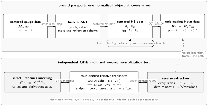
The complete round trip. The upper lane fixes the finite-Omega representative, carries centered masses through AGT, and takes the declared NS path to a standard Heun equation. The connection matrix still needs the internal lift, endpoint derivatives, unit-leading frames, and path. The lower lane supplies independent Frobenius and Wronskian checks; two ratios in each matrix direction reconstruct $F_0$ and $F_t$ and distinguish an internal-core mismatch from endpoint truncation.

The block prediction is an actual pair of connection formulae

Substitution gives

$$C_{t0}^{[2]} \approx \begin{pmatrix} 0.6852142054&0.5321841143 \\ 1.0470983914&-0.6945967755 \end{pmatrix}.$$

Because columns label source germs, this means

$$\begin{aligned} H_{0,-} \approx{}& 0.6852142054\,H_{t,-} \\ &+ 1.0470983914\,H_{t,+}, \end{aligned}$$

and

$$\begin{aligned} H_{0,+} \approx{}& 0.5321841143\,H_{t,-} \\ &- 0.6945967755\,H_{t,+}. \end{aligned}$$

The approximation symbol refers to truncation of the accessory and endpoint derivatives through $t^2$. It does not refer to an arbitrary normalization of the local germs: each of the four germs has leading coefficient one in its declared local coordinate.

A change from $t-z$ to $z-t$ would multiply $H_{t,+}$ by a branch phase and therefore left-multiply $C_{t0}$ by an inverse diagonal matrix. Winding the path around zero or $t$ produces the general two-sided covariance law

$$C_{t0}^{\mathrm{new}} = M_t^{-1}C_{t0}M_0.$$

Raw entries from different paths should never be compared before this transport is applied.

Direct Frobenius matching checks every entry

Now forget the connection formula and solve the displayed Heun equation directly. Generate the two Frobenius series at zero and the two series at $t$, keeping the same unit-leading powers. At the ordinary matching point

$$z_\ast=\frac t2=\frac1{50},$$

form the two fundamental matrices from values and derivatives and compute

$$C_{t0}^{\mathrm{Frob}} = \Phi_t(z_\ast)^{-1}\Phi_0(z_\ast).$$

High-precision evaluation gives

$$C_{t0}^{\mathrm{Frob}} \approx \begin{pmatrix} 0.6852083269&0.5321827959 \\ 1.0471097736&-0.6945959089 \end{pmatrix}.$$

The comparison is

Entry	Block through $t^2$	Direct Frobenius	Relative error
$(C_{t0})_{--}$	$0.6852142054$	$0.6852083269$	$8.58\times10^{-6}$
$(C_{t0})_{-,+}$	$0.5321841143$	$0.5321827959$	$2.48\times10^{-6}$
$(C_{t0})_{+,-}$	$1.0470983914$	$1.0471097736$	$1.09\times10^{-5}$
$(C_{t0})_{+,+}$	$-0.6945967755$	$-0.6945959089$	$1.25\times10^{-6}$

Moving $z_\ast$ within the common convergence lens leaves the matrix unchanged: matching at $t/2$ and $t/3$ changes it by only $1.88\times10^{-29}$ in an 80-digit, 160-term run. Repeating the comparison for $t=0.08,0.04,0.02,0.01$ shows level-two errors proportional to $t^3$. This scaling is an important consistency check: the accessory and both endpoint derivatives must be truncated at the same sewing level.

An instructive ablation is to set $F_0=F_t=0$ while leaving every other factor unchanged. The determinant still passes, but the maximum entrywise error rises from $1.09\times10^{-5}$ to $6.83\times10^{-3}$. Endpoint derivatives are therefore observable in individual connection coefficients even though the Wronskian cannot see them.

The calculation is reproducible with general-heun-connection-check.py. The script constructs both local recurrences, matches values and derivatives, assembles the block prediction, and evaluates the Wronskian determinant independently. Run it with --terms 160 --dps 80 and --show-reverse --show-ablation --check-second-point to reproduce the three additional diagnostics used on this page at the stated precision.

Abel’s identity supplies an exact checksum

For the declared unit-leading bases, the general determinant formula is

$$\det C_{t0} = \frac{1-\gamma_{\mathrm H}} {\epsilon_{\mathrm H}-1} t^{\epsilon_{\mathrm H}-\gamma_{\mathrm H}} (1-t)^{-\delta_{\mathrm H}}.$$

Here $\gamma_{\mathrm H}=\epsilon_{\mathrm H}=2/3$, so

$$\boxed{ \det C_{t0} = -\left(\frac{25}{24}\right)^{4/5} \approx -1.03319670758601. }$$

The fusion construction gives the same result because

$$\det M_{\mathrm{fr}} = -\frac{a_0}{a_t} =-1,$$

and

$$\frac{\det D_0}{\det D_t} =(1-t)^{-4/5}.$$

The endpoint derivatives cancel exactly. This makes the determinant a strong but incomplete test: it detects a wrong target power or gamma factor in many implementations, but it is invariant under transpose and cannot detect a pair of opposite diagonal rescalings whose determinants cancel. The four-entry Frobenius comparison remains necessary.

The numerical matrix reconstructs the endpoint generator

The direct matrix contains more information than its determinant. Divide entries in a common target row to isolate $F_0$, and divide entries in a common source column to isolate $F_t$. Write

$$C_{t0} = \begin{pmatrix} C_{--}&C_{-,+} \\ C_{+,-}&C_{+,+} \end{pmatrix}.$$

The two independent reconstructions of $F_0$ are

$$\begin{aligned} F_0^{(-)} &= \Log\left[ \frac{ C_{-,+}\mathcal M_{--} }{ t^{1-\gamma_{\mathrm H}} C_{--}\mathcal M_{+,-} } \right], \\ F_0^{(+)} &= \Log\left[ \frac{ C_{+,+}\mathcal M_{-,+} }{ t^{1-\gamma_{\mathrm H}} C_{+,-}\mathcal M_{++} } \right]. \end{aligned}$$

Likewise,

$$\begin{aligned} F_t^{(-)} &= -\Log\left[ \frac{ t^{1-\epsilon_{\mathrm H}} C_{+,-}\mathcal M_{--} }{ C_{--}\mathcal M_{-,+} } \right], \\ F_t^{(+)} &= -\Log\left[ \frac{ t^{1-\epsilon_{\mathrm H}} C_{+,+}\mathcal M_{+,-} }{ C_{-,+}\mathcal M_{++} } \right]. \end{aligned}$$

All four ratios are positive on the chosen real branch, so the real logarithm is selected. On a complex continuation the logarithm sheet is additional data and each answer is defined modulo $2\pi\ii$.

Equivalently, strip the known core and endpoint powers:

$$R_{rs} := \frac{ (C_{t0})_{rs} }{ (1-t)^{-(1-\theta_1)/2} t^{[\theta_0(s+1)-\theta_t(r+1)]/2} (M_{\mathrm{fr}})_{rs} }.$$

For an untruncated matrix and fusion core on the same internal branch,

$$R_{rs} = \exp\left[ \frac{sF_0-rF_t}{2} \right],$$

and the two exact compatibility checks are

$$R_{--}R_{++}=1, \qquad R_{-,+}R_{+,-}=1.$$

Substituting $C_{t0}^{\mathrm{Frob}}$ gives

$$\begin{aligned} F_0^{(-)} &\approx0.0067855890, & F_0^{(+)} &\approx0.0067673694, \\ F_t^{(-)} &\approx-0.0068399622, & F_t^{(+)} &\approx-0.0068217425. \end{aligned}$$

The redundant values differ by about $1.82\times10^{-5}$. No endpoint series was used in forming these ratios. The residual instead detects that the direct matrix solves the equation with $\mathfrak q_{\mathrm H}^{[2]}$, whose exact composite monodromy is not quite the intended $a=3/10$ formal branch.

Indeed, in the natural determinant-one scalar half-density lifts, put

$$L_f := -\ee^{-\pi\ii\theta_f} \operatorname{diag} \left( 1,\ee^{2\pi\ii\theta_f} \right).$$

The row-frame direction gives the exact composite trace of the displayed truncated equation as

$$\begin{aligned} T_{0t}^{[2]} &= \operatorname{tr} \left[ L_0 (C_{t0}^{\mathrm{Frob}})^{-1} L_t C_{t0}^{\mathrm{Frob}} \right] \\ &\approx0.618047568855109. \end{aligned}$$

This effective trace differs from the untruncated target trace $(\sqrt5-1)/2\approx0.618033988749895$.

Solving $T_{0t}^{[2]}=-2\cos(\pi\theta_{0t}^{\mathrm{eff}})$ on the lift near $3/5$—or enforcing equality of the two $F_0$ ratios—recovers

$$\begin{aligned} a_{\mathrm{eff}} &\approx0.300001136285459, \\ \theta_{0t}^{\mathrm{eff}} &=2a_{\mathrm{eff}} \approx0.600002272570917. \end{aligned}$$

Rebuilding the fusion core at $a_{\mathrm{eff}}$ makes the redundant reconstructions agree to the working precision:

$$\begin{aligned} F_0^{\mathrm{eff}} &\approx0.006782301436043, \\ F_t^{\mathrm{eff}} &\approx-0.006825030070709. \end{aligned}$$

The remaining differences between these exact equation-first values and the level-two endpoint predictions

$$F_0^{[2]} \approx0.0067794872, \qquad F_t^{[2]} \approx-0.0068205128.$$

are attributable, to the displayed accuracy, to omitted higher endpoint levels. Re-evaluating the level-two jets at $a_{\mathrm{eff}}$ changes them by only about $2.9\times10^{-12}$. The two effects should not be conflated: disagreement between redundant ratios tests the accessory/internal-core match, while displacement of their common value from $F_0^{[2]},F_t^{[2]}$ tests endpoint truncation.

This redundancy is a practical diagnostic. If the two extractions of one derivative disagree at order unity, likely causes are a transpose, a wrong $t-z$ phase, an inconsistent block prefactor, or an incorrect accessory branch. If one denominator is near zero, the corresponding ratio is ill-conditioned; use the other row or column rather than dividing by a small connection entry.

Return to the two right-flavor derivatives

The centered variables obey

$$p_0=\frac{M_3-M_4}{2}, \qquad p_t=\frac{M_3+M_4}{2}.$$

For the matched endpoint generator,

$$\begin{aligned} \partial_{M_3}\widehat{\mathcal W} &= \frac{F_0+F_t}{2}, \\ \partial_{M_4}\widehat{\mathcal W} &= \frac{F_t-F_0}{2}. \end{aligned}$$

At level two this yields

$$\partial_{M_3}\widehat{\mathcal W}^{[2]} = -\frac1{48750}, \qquad \partial_{M_4}\widehat{\mathcal W}^{[2]} = -\frac{17}{2500}.$$

These are derivatives of the declared matched endpoint generator, not of an unspecified raw localization functional. Adding a $t$-independent mass function leaves the accessory unchanged but shifts these derivatives and therefore rescales columns or rows of the connection matrix.

The dictionary can be run backward

Suppose the starting object were instead the displayed Heun equation and its directly computed $C_{t0}$. The reverse reconstruction proceeds as follows.

1. Read $\theta_0=1-\gamma_{\mathrm H}=1/3$, $\theta_t=1-\epsilon_{\mathrm H}=1/3$, $\theta_1=1-\delta_{\mathrm H}=1/5$, and $\theta_\infty=\alpha_{\mathrm H}-\beta_{\mathrm H}=1/5$, retaining the declared exponent ordering.
2. Decide which inverse is intended. The formal passport retains $\theta_{0t}=3/5$ through level two. The exact displayed truncated ODE instead gives $\theta_{0t}^{\mathrm{eff}}\approx0.600002272570917$ from composite monodromy or four-entry compatibility. Either trace inverse still allows $\theta_{0t}\mapsto\pm\theta_{0t}+2n$.
3. Restore the first-plane polarization and $\hbar=5/2$. Then $p_f=\hbar\theta_f/2$ and $a_{\mathrm C}=\hbar\theta_{0t}/2=3/4$ on the intended formal branch after choosing the positive Weyl representative. Equation-first inversion of the truncated ODE gives the nearby effective value $a_{\mathrm C}^{\mathrm{eff}}\approx0.750002840713646$.
4. Invert the flavor pairing to obtain $(M_1,M_2,M_3,M_4)=(1/2,0,5/6,0)$.
5. Choose $\epsilon_2=2/5$, the positive $\varepsilon_\star=1$, and the same matter orientation. Reinsert $\epsilon_\Sigma/2$ to recover the finite-Omega printed masses and use $\alpha_f=Q_{\mathrm L}/2+p_f/\varepsilon_\star$ to recover the four external Liouville momenta. Recover the internal momentum separately from $\alpha_{0t}=Q_{\mathrm L}/2+a_{\mathrm C}/\varepsilon_\star$.
6. Use the four connection-entry ratios to reconstruct $F_0,F_t$ and test the endpoint normalization. Restore their logarithm branches.
7. Restore $\beta_{0t}$, the local coordinates $z$ and $t-z$, and the row-frame direction. Without these, the four matrix entries are not comparable objects.

Every inverse step needs information that a square, trace, accessory, or connection determinant forgot. The reconstruction is therefore a passport, not a one-line equality among theories.

Reversible passport for the complete example

Map	Forward direction	Reverse direction	Convention, exclusion, and source
Omega background $\leftrightarrow$ Liouville coupling	$b^2=\epsilon_2/\epsilon_1$, $\varepsilon_\star^2=\epsilon_1\epsilon_2$, $Q_{\mathrm L}=b+b^{-1}$	Restore the ordered Omega planes, the sign of $\varepsilon_\star$, and one root of $b+b^{-1}=Q_{\mathrm L}$	The exchange $b\leftrightarrow b^{-1}$ also exchanges the degenerate probe and NS polarization; AGGTV §§1.2, 2.2
Centered gauge masses $\leftrightarrow$ puncture masses	Pair $M_{1,2}$ into $p_\infty,p_1$ and $M_{3,4}$ into $p_t,p_0$	Invert the two sum–difference systems	Fix flavor ordering, matter orientation, and centered mass scheme; AGT §3.2
Centered mass $\leftrightarrow$ Liouville momentum	$\alpha_f=Q_{\mathrm L}/2+p_f/\varepsilon_\star$	$p_f=\varepsilon_\star(\alpha_f-Q_{\mathrm L}/2)$	Restore square-root branch and reflection representative; AGT §3.2
Puncture mass $\leftrightarrow$ oper exponent	$\theta_f=2p_f/\hbar$	$p_f=\hbar\theta_f/2$	First Omega plane and $V_{-b/2}$ probe; endpoint resonance requires a logarithmic or limiting basis; AGGTV §§1.2, 2.2
Coulomb coordinate $\leftrightarrow$ internal lift	$a=a_{\mathrm C}/\hbar=\theta_{0t}/2$	Choose the exponent lift and Weyl sign	Trace inversion is ramified at $\operatorname{tr}M_{0t}=\pm2$; Jeong–Nekrasov §6
Internal lift $\leftrightarrow$ accessory branch	$\partial_t\widehat f$ plus scalar-gauge contacts gives $\mathfrak q_{\mathrm H}(t)$	Invert locally in $a$ or compute composite monodromy	Requires one normalized full block and a noncritical branch; Litvinov et al. §2 and Bonelli et al. §§3.1, 4.1
Fusion and endpoint data $\leftrightarrow$ connection matrix	$C_{t0}=D_t^{-1}M_{\mathrm{fr}}D_0$	Entry ratios recover $F_0,F_t$ when denominators are nonzero	Fix unit-leading germs, path, row/column convention, block normalization, and logarithm sheets; Bonelli et al. §4.1
Local frames $\leftrightarrow$ direct matrix	$C_{t0}=\Phi_t^{-1}\Phi_0$ at a common ordinary point	Recover one frame from the other only after its normalization is supplied	Frobenius disks must overlap or continuation must be subdivided; DLMF §31.3
Matrix $\leftrightarrow$ determinant	Take $\det C_{t0}$	A determinant never reconstructs four entries	Abel’s identity fixes the Wronskian ratio; DLMF §1.13(i), Eq. (1.13.5)

The source column deliberately mixes primary correspondence papers with the DLMF’s convention references. AGT supplies the finite-Omega block and mass map; the degenerate heavy–light construction supplies the formal connection formula; ordinary ODE theory supplies the independent local solution and determinant checks.

Exceptional loci and claims not made

Locus or omitted datum	What fails	Required replacement
$\theta_0\in\mathbb Z$ or $\theta_t\in\mathbb Z$	The generic two-power unit-leading frame and gamma kernel can be singular	A logarithmic or compatible limiting basis and a recomputed connection matrix
Internal Kac divisor	The inverse-Gram conformal-block chart is meromorphic	A compatible quotient block or analytic limiting prescription
$\operatorname{tr}M_{0t}=\pm2$	The internal trace inverse loses semisimple/Jordan and exponent-lift data	Full conjugacy class, eigenline or Jordan flag, and a limiting lift
$\partial_a\mathfrak q_{\mathrm H}=0$	Accessory-to-internal inversion ramifies	Another local coordinate or a ramified branch parameter
A connection entry used in a ratio vanishes	One reverse derivative formula is ill-conditioned or undefined	Use its redundant row or column, or solve the full factorization
$t\in\{0,1,\infty\}$	The regular four-puncture chart degenerates	A controlled sewing or confluence limit with rescaled parameters
Path crosses a cut or winds a puncture	Raw entries acquire endpoint monodromy factors	Apply $M_t^{-1}C_{t0}M_0$ with declared phases
Continuation beyond the small-$t$ disk	The displayed truncation has no automatic accuracy guarantee	Higher levels, analytic continuation, or direct numerical matching
A boundary condition is imposed	A spectral problem is created, but no eigenvalue condition follows from the matrix alone	Select the relevant entry or Wronskian and prove the boundary equivalence
Nonperturbative gauge completion is requested	The formal NS series is insufficient by itself	Specify the chamber and completion appropriate to the physical problem

In particular, no closed WKB period was needed to compute this local regular connection matrix. The previous page’s cycle dictionary remains essential if one replaces the internal monodromy label by a quantum period or imposes a global spectral condition. That further step is conditional on the operator, lattice, polarization, and resummation passport recorded there.

A minimal normalization certificate

Before quoting the numerical matrix outside this page, attach all ten items:

1. Equation: standard Heun with singularities $(0,t,1,\infty)$ and the displayed accessory.
2. Parameter branch: $t=1/25$ and the internal lift $a=3/10$.
3. Source frame: $(1+O(z),z^{1/3}[1+O(z)])$.
4. Target frame: $(1+O(t-z),(t-z)^{1/3}[1+O(t-z)])$.
5. Path: the real interval from each endpoint into $0<z<t$ with no winding.
6. Direction: $\boldsymbol H_0=\boldsymbol H_tC_{t0}$, target rows and source columns.
7. Block scheme: unit-leading, Heisenberg-stripped $\widehat f$ with $a$ held fixed under external derivatives.
8. Gauge scheme: centered $M_i$ fixed on the first-plane NS path, with the $V_{-b/2}$ probe, flavor pairing, and matter orientation fixed.
9. Accuracy statement: accessory and endpoint data through $t^2$; direct Frobenius solution of that truncated equation.
10. Checks: four-entry match, matching-point independence, redundant derivative inversion, and exact Wronskian determinant.

Removing any one of items 2–8 changes or underdetermines at least one matrix entry. Items 9–10 prevent a formal approximation from being reported with unjustified precision.

Common pitfalls

Freezing the wrong masses. Printed $\mu_i$ include $\epsilon_\Sigma/2$ and move along the centered NS path. Freeze $M_i$ or $p_f$ when the local exponents are intended to stay fixed.

Calling the fusion core the connection matrix. The gamma kernel lacks endpoint derivatives and coordinate powers. The correct unit-leading object is $D_t^{-1}M_{\mathrm{fr}}D_0$.

Reading rows as source branches. In $\boldsymbol H_0=\boldsymbol H_tC_{t0}$, columns are source branches and rows are target branches. This is why the sign-indexed fusion array is transposed when arranged as $M_{\mathrm{fr}}$.

Differentiating after accessory inversion. $F_0$ and $F_t$ are external derivatives at fixed internal lift $a$. Differentiating the composite $a(\mathfrak q_{\mathrm H},t)$ introduces a spurious chain-rule contribution.

Mixing $z-t$ with $t-z$. Their fractional powers differ by a path phase. A formula copied between the two local coordinates must transform the target frame.

Trusting only the determinant. Opposite endpoint rescalings can leave the determinant correct while changing every column or row. Check all four entries and reconstruct both derivatives.

Using inconsistent sewing orders. Truncating the accessory at one order and the endpoint derivatives at another destroys the expected $O(t^{N+1})$ error law.

Turning a connection formula into a spectrum. A spectrum appears only after a boundary condition selects a vanishing entry or boundary Wronskian. No such condition has been imposed here.

Exercises

1. Reconstruct the finite-Omega representative

Starting from the centered $M_i$, $\epsilon_1=5/2$, and $\epsilon_2=2/5$, recompute the four printed masses and the five Liouville momenta.

Solution

Since $\epsilon_\Sigma/2=29/20$,

$$\mu_i=M_i+\frac{29}{20},$$

which gives

$$\left( \frac{39}{20}, \frac{29}{20}, \frac{137}{60}, \frac{29}{20} \right).$$

Here $Q_{\mathrm L}/2=29/20$ and $\varepsilon_\star=1$. Adding $p_\infty=p_1=1/4$, $p_t=p_0=5/12$, and $a_{\mathrm C}=3/4$ gives respectively $17/10,17/10,28/15,28/15$, and $11/5$.

2. Diagnose the wrong NS path

Hold the four finite-Omega $\mu_i$ fixed while sending $\epsilon_2\to0$. Compute the endpoint centered masses and explain why this does not reproduce the declared oper passport.

Solution

At the endpoint $\epsilon_\Sigma/2=5/4$. Holding the printed masses fixed gives

$$(M_1,M_2,M_3,M_4) = \left( \frac7{10}, \frac15, \frac{31}{30}, \frac15 \right),$$

not $(1/2,0,5/6,0)$. Common shifts leave the difference coordinates $p_\infty$ and $p_0$ unchanged, but they change the sum coordinates $p_1$ and $p_t$. The full puncture passport and the normalized contact terms therefore belong to a different path.

3. Recover the Heun parameters

Use the four oriented exponent differences to derive $\gamma_{\mathrm H},\delta_{\mathrm H},\epsilon_{\mathrm H}, \alpha_{\mathrm H},\beta_{\mathrm H}$ and verify the Fuchs relation.

Solution

Substitution into the exponent dictionary gives

$$\left( \gamma_{\mathrm H}, \delta_{\mathrm H}, \epsilon_{\mathrm H}, \alpha_{\mathrm H}, \beta_{\mathrm H} \right) = \left( \frac23,\frac45,\frac23,\frac23,\frac7{15} \right).$$

Both sides of the Fuchs relation equal $32/15$.

4. Derive the first reverse ratio

Starting from the explicit entry formula, divide $C_{-,+}$ by $C_{--}$ and solve for $F_0$. Why do the two target-row extractions from the direct matrix disagree slightly when the core is fixed at $a=3/10$?

Solution

The common factor $(1-t)^{-\delta_{\mathrm H}/2}$ and all $F_t$ dependence cancel:

$$\frac{C_{-,+}}{C_{--}} = t^{1-\gamma_{\mathrm H}} \frac{\mathcal M_{+,-}}{\mathcal M_{--}} \ee^{F_0}.$$

Taking the declared logarithm gives $F_0^{(-)}$ in the text.

The direct matrix is exact for the ODE with the truncated accessory $\mathfrak q_{\mathrm H}^{[2]}$. That equation lies on the nearby leaf $a_{\mathrm{eff}}\approx0.300001136285459$, not exactly on the intended untruncated leaf $a=3/10$. Rebuilding the gamma core at $a_{\mathrm{eff}}$ makes the two target-row extractions agree; their remaining displacement from $F_0^{[2]}$ measures omitted endpoint levels.

5. Check the determinant without blocks

Use the unit-leading Wronskians at zero and $t$ to derive the determinant at $t=1/25$.

Solution

Abel’s identity gives

$$\det C_{t0} = \frac{1-\gamma_{\mathrm H}} {\epsilon_{\mathrm H}-1} t^{\epsilon_{\mathrm H}-\gamma_{\mathrm H}} (1-t)^{-\delta_{\mathrm H}}.$$

The first ratio is $-1$, the $t$ power is one, and $(1-t)^{-4/5}=(25/24)^{4/5}$. Hence the result is $-(25/24)^{4/5}$.

6. Change the target local coordinate

Continue above the real axis and replace $(t-z)^{1/3}$ by $(z-t)^{1/3}$. Find the transformation of $C_{t0}$.

Solution

Above the cut,

$$(z-t)^{1/3} = \ee^{\pi\ii/3}(t-z)^{1/3}.$$

Thus the new target frame is

$$\boldsymbol H_t^{\mathrm{new}} = \boldsymbol H_t \operatorname{diag}(1,\ee^{\pi\ii/3}).$$

Keeping the source frame fixed gives

$$C_{t0}^{\mathrm{new}} = \operatorname{diag}(1,\ee^{-\pi\ii/3})C_{t0}.$$

7. Separate the relative path from the composite cycle

Why does the connection path $\beta_{0t}$ not determine the composite trace or the SW A-period by itself?

Solution

$\beta_{0t}$ is open and carries endpoint-normalized transport. The composite trace belongs to a closed based loop on the punctured base, while the SW period belongs to a primitive class on a spectral cover. Closing or lifting the path requires a base point, sheet, detours, integral-lattice saturation, and an $SL(2)$ lift. None is encoded by the open interval alone.

8. Turn the matrix into a boundary condition

Suppose a boundary problem selects $H_{0,-}$ at zero and requires the coefficient of $H_{t,+}$ to vanish. Which matrix entry is the boundary function in the present direction? Is it zero in the example?

Solution

The first column expands $H_{0,-}$. Its $H_{t,+}$ coefficient is the target-plus/source-minus entry $C_{+,-}$. Numerically it is about $1.0471097736$, so this parameter point does not satisfy the proposed boundary condition.

References

• L. F. Alday, D. Gaiotto, and Y. Tachikawa, “Liouville Correlation Functions from Four-Dimensional Gauge Theories”, Letters in Mathematical Physics 91 (2010), 167–197. Section 3.2 and equations (3.5)–(3.13) give the regular four-point block, mass pairing, internal Coulomb map, and Heisenberg factor used to define the finite-Omega representative. The uniform centering $M_i=\mu_i-\epsilon_\Sigma/2$, dimensional restoration, and exact flavor ordering displayed here are the book’s declared translation of that convention.
• L. F. Alday, D. Gaiotto, S. Gukov, Y. Tachikawa, and H. Verlinde, “Loop and Surface Operators in N=2 Gauge Theory and Liouville Modular Geometry”, Journal of High Energy Physics 01 (2010) 113. Sections 1.2 and 2.2 propose the correspondence between the two Omega-plane defects and the two degenerate fields and give the null relation and adjacent fusion rule behind the first-plane probe.
• A. Litvinov, S. Lukyanov, N. Nekrasov, and A. Zamolodchikov, “Classical Conformal Blocks and Painlevé VI”, Journal of High Energy Physics 07 (2014) 144. Equations (1.8), (2.7)–(2.10), and (2.13)–(2.19) relate the normalized four-point classical block to the four-pole oper, its accessory, and the composite monodromy data.
• S. Jeong and N. Nekrasov, “Opers, Surface Defects, and Yang–Yang Functional”, Advances in Theoretical and Mathematical Physics 24 (2020), 1789–1916. Equations (3.14)–(3.23), (6.9)–(6.12), and (6.18)–(6.26) give the finite-Omega defect identity, NS oper, composite trace, normalized generating function, and prefactor, one-loop, and boundary-term qualifications used in the gauge-to-oper and reverse-derivative lanes.
• G. Bonelli, C. Iossa, D. Panea Lichtig, and A. Tanzini, “Irregular Liouville Correlators and Connection Formulae for Heun Functions”, Communications in Mathematical Physics 397 (2023), 635–727; version-of-record DOI. In arXiv v3 numbering, equation (2.1.7), equations (3.1.22)–(3.1.30), equations (4.1.1)–(4.1.9) and (4.1.16)–(4.1.17), and Appendix C.1 supply the fusion kernel, classical endpoint dressings, standard-Heun dictionary, unit-leading germs, connection formula, and accessory series. The indexed kernel and Wronskian audit avoid the apparent lower-right gamma-factor typo discussed on the Chapter 7 derivation page; the exact accessory relation also avoids the defective shortcut in arXiv v3 equation (4.1.18). The corresponding publisher numbers are (4.1.15)–(4.1.16) for the connection components and (4.1.17) for the shortcut.
• O. Lisovyy and A. Naidiuk, “Perturbative Connection Formulas for Heun Equations”, Journal of Physics A: Mathematical and Theoretical 55 (2022) 434005; version-of-record DOI. Corollary 3.2 gives the Schäfke–Schmidt coefficient extraction, while Theorem B and Section 4.2 separate exact continued-fraction ODE statements from finite-order checks of the formal classical-block relation. Section 5 states the remaining global analytic caveat.
• M. Piątek and A. R. Pietrykowski, “Solving Heun’s Equation Using Conformal Blocks”, Nuclear Physics B 938 (2019), 543–570. Sections 2–4 provide an independent normalization-aware classical-block construction of Heun accessory data and local solutions.
• NIST Digital Library of Mathematical Functions, §1.13(i), Eq. (1.13.5), §31.2, and §31.3. These sections fix Abel’s identity, the standard general-Heun equation and exponent ledger, and the normalized local Heun solution with its exceptional parameters.