Isomonodromic and Conformal-Block Formulations

The preceding page defined the physical spectrum by two primary objects, $E_{\mathrm{ang}}(A,\omega)$ and $E_{\mathrm{rad}}(A,\omega)$. An isomonodromic formulation does not replace those boundary functions by the slogan “set tau to zero.” It translates their endpoint lines into framed monodromy data, embeds each Heun equation into a chosen Painlevé family, and reconstructs the physical accessory parameter in that chart.

Kerr–de Sitter is the clean regular-singularity laboratory. Its angular and radial equations are both general Heun equations, hence each admits a Painlevé VI (PVI) inverse problem. The angular and radial problems share the same separation constant and frequency, so only their coupled solution can be a quasinormal mode (QNM). Central-charge-one and classical conformal blocks then offer different ways to compute parts of this inverse map; they are not interchangeable names for one object.

First reading

Follow boundary line → framed monodromy → Heun collision slice → neighboring tau zero plus base-tau derivative → coupled Kerr–de Sitter equations. The Fourier-block chart, confluence, and resonant qualifications may wait for a second pass. Readers already fluent in the PVI inverse dictionary may move directly to the named Kerr–de Sitter application.

Status ledger

Statement	Status and scope
Boundary Wronskian equals a selected connection entry up to a nonzero factor	Exact in the endpoint frames of the preceding page
Selected regular endpoint lines imply a framed common-eigenline condition	Exact for the declared local eigenlines
One composite trace identifies the selected boundary branch	False without extra flag or continuation data; the trace sees a union of branches
General Heun as a PVI collision slice	Exact in the displayed cyclic component, integer lifts, and finite-momentum chart
Neighboring tau zero and base-tau accessory derivative	Exact on the stated nonresonant Schlesinger patch with nonzero base tau
Generic PVI central-charge-one Fourier expansion	Exact locally, up to a nonzero time-independent tau normalization
Classical-block accessory derivative	Branchwise semiclassical statement in its declared oper normalization
Scalar Kerr–de Sitter Heun operators, exponents, and accessories below	Exact for the conformally coupled scalar in the displayed source convention
Replacing selected Kerr–de Sitter connection entries by composite lifts	Source-calibrated candidate reduction; angular data are resonant, and direct selected-connection or Wronskian validation remains necessary
Small-rotation and near-Nariai accessory expansions	Controlled asymptotic charts, not one uniform expansion
Flat Kerr Painlevé V formulation	Requires operator-level confluence and wild monodromy; it is not obtained by direct substitution in PVI formulas
A tau zero is a QNM	Not true without the boundary, accessory, angular, sheet, and validation gates

The translation is a chain of gated maps

At fixed black-hole parameters and mode labels, the primary spectral system is

$$\begin{aligned} E_{\mathrm{ang}}(A,\omega)&=0, \qquad E_{\mathrm{rad}}(A,\omega)=0. \end{aligned}$$

Every later representation must recover this same local zero set, including its multiplicities, after all auxiliary monodromy variables have been eliminated. The logical chain is

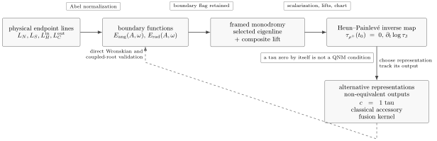
Every arrow carries data. The neighboring tau zero selects a Heun collision slice, while a generally different base tau reconstructs the accessory. A tau zero by itself is therefore not a QNM condition. The final box lists three alternative representations with non-equivalent outputs, not three successive steps.

The objects along this chain answer different questions:

Object	Question answered	Information still missing
$E_B$	Do the two selected endpoint lines coincide?	No monodromy representation is needed
Selected connection entry	Which coefficient of an unwanted endpoint vector vanishes?	Depends on ordered, normalized endpoint frames
Framed monodromy locus	Which marked monodromy representation preserves the selected line?	The physical accessory equation
Neighboring tau zero	Does the apparent scalar point collide on the chosen Heun branch?	The physical boundary line and accessory
Base-tau derivative	Which Heun accessory belongs to that monodromy data?	A normalized connection coefficient
Conformal-block expansion	How can the tau, accessory, or connection kernel be represented in a chosen chart?	The other gates and an ODE validation

The safest direction of reasoning is left to right for construction and right to left for validation.

Boundary alignment is framed monodromy

First suppose the two relevant endpoints are regular singular points and their local monodromies are diagonalizable. Use the book convention

$$\operatorname{tr}M_j=2\cos(\pi\vartheta_j),$$

so the two local eigenvalues are $\ee^{\pm\pi\ii\vartheta_j}$. Let the physical line at endpoint $j$ select the sign $s_j\in\{+1,-1\}$. If the selected lines at $L$ and $R$ coincide, a nonzero vector $v$ obeys

$$\begin{aligned} M_Lv&=\ee^{\pi\ii s_L\vartheta_L}v, \qquad M_Rv=\ee^{\pi\ii s_R\vartheta_R}v. \end{aligned}$$

In a basis beginning with $v$, both matrices are triangular. Their product therefore has trace

$$\operatorname{tr}(M_LM_R) = 2\cos\left[ \pi(s_L\vartheta_L+s_R\vartheta_R) \right].$$

This is a necessary composite-monodromy equation for the boundary intersection. It becomes sufficient only after the common eigenline is identified with the selected endpoint vectors. A trace forgets that flag: exchanging one local eigenline can give the same trace, and the periodicity of cosine retains all integer lifts. Thus a composite trace normally describes a union of boundary branches.

At an irregular endpoint, local monodromy is even less information. The physical vector also depends on Stokes sectors, lateral continuation, and Stokes matrices. The correct replacement is a framed wild-monodromy condition, not an unadorned trace.

Convert the black-hole convention once

The Kerr–de Sitter literature used below writes half exponent differences $\widehat\theta_j$ and defines

$$\begin{aligned} \operatorname{tr}M_j &=2\cos(2\pi\widehat\theta_j), \end{aligned}$$

while its composite coordinate satisfies

$$\operatorname{tr}(M_jM_k) = -2\cos(2\pi\widehat\sigma_{jk}).$$

A convenient scalar-to-system lift conversion to the book convention is

$$\begin{aligned} \vartheta_j&=2\widehat\theta_j, \qquad \varsigma_{jk}=2\widehat\sigma_{jk}+1, \end{aligned}$$

because then

$$\operatorname{tr}(M_jM_k) =2\cos(\pi\varsigma_{jk}).$$

The added unit is the central shift between the scalar-oper and traceless system lifts. Other representatives differing by an even integer have the same trace, but the displayed representative is the one used with the Heun–PVI shift table below. Reducing it modulo $2$ before selecting a boundary branch loses the overtone and continuation data.

A generic PVI scalarization has an apparent fifth point

Write the target general Heun equation as

$$\begin{aligned} y'' &+ \left( \frac{1-\vartheta_0}{z} +\frac{1-\vartheta_1}{z-1} +\frac{1-\vartheta_t}{z-t_0} \right)y' \\ &+ \frac{\alpha_{\mathrm H}\beta_{\mathrm H}z-q_{\mathrm H}} {z(z-1)(z-t_0)}y =0. \end{aligned}$$

The finite local exponent pairs are $(0,\vartheta_0)$, $(0,\vartheta_1)$, and $(0,\vartheta_t)$. A traceless two-by-two Fuchsian system with poles at $0,t,1,\infty$ carries the full two-dimensional monodromy manifold. Eliminating one component with a generic cyclic vector does not immediately give this Heun equation. It gives a scalar equation with an additional point $z=\lambda(t)$:

$$y'' + \left[ \sum_{j\in\{0,t,1\}} \frac{p_j}{z-j} -\frac1{z-\lambda(t)} \right]y' +V(z;\lambda,\mu,t)y =0.$$

The residue data make $z=\lambda(t)$ apparent, so its local solutions have trivial projective monodromy. The Darboux pair $(\lambda,\mu)$ evolves by the PVI Hamiltonian equations. The marked Heun equation appears only on a collision slice such as

$$t=t_0, \qquad \lambda(t_0)=t_0,$$

with the conjugate momentum finite in the chart used here. Another cyclic component, another collision pole, or the other momentum branch changes the integer shifts and printed accessory formula.

In the displayed finite-momentum chart the second collision datum is

$$\mu(t_0)=-\frac{K_0}{\theta_t}, \qquad \theta_t=\vartheta_t-1\ne0.$$

Thus the chart itself fails at $\vartheta_t=1$ and must be replaced there.

The deformation system carries shifted lifts

Let $\rho_{\mathrm H}$ denote the target-Heun lifts and $\rho$ the PVI deformation lifts in the collision convention of Chapter 5. They are related by

$$\begin{array}{c|cccc} &\theta_0&\theta_t&\theta_1&\theta_\infty\\ \hline \rho_{\mathrm H} &\vartheta_0&\vartheta_t&\vartheta_1&\vartheta_\infty\\ \rho &\vartheta_0&\vartheta_t-1&\vartheta_1&\vartheta_\infty+1 \end{array}$$

and

$$\begin{array}{c|ccc} &\sigma_{0t}&\sigma_{1t}&\sigma_{01}\\ \hline \rho_{\mathrm H} &\varsigma_{0t}&\varsigma_{1t}&\varsigma_{01}\\ \rho &\varsigma_{0t}-1&\varsigma_{1t}-1&\varsigma_{01}. \end{array}$$

These shifts change the marked scalar equation even though some projective traces are unchanged. A formula evaluated at the unshifted Heun tuple is a different formula.

Two tau functions perform two different jobs

Let $A_j$ be the system residues and

$$B_j=A_j-\frac{\theta_j}{2}I$$

their traceless parts. The Jimbo–Miwa–Ueno (JMU) tau function in this representative satisfies

$$\begin{aligned} \frac{\partial}{\partial t} \log\tau_{\mathrm J}(\rho;t) &= \frac{\operatorname{tr}(B_tB_0)}{t} + \frac{\operatorname{tr}(B_tB_1)}{t-1}. \end{aligned}$$

On the finite-momentum collision branch, the compact Heun accessory is

$$\begin{aligned} K_0 = \left[ \frac{\partial}{\partial t} \log\tau_{\mathrm J}(\rho;t) -\frac{\theta_0\theta_t}{2t} -\frac{\theta_1\theta_t}{2(t-1)} \right]_{t=t_0}. \end{aligned}$$

Consequently the standard Heun parameter is

$$\begin{aligned} q_{\mathrm H} ={}& t_0\alpha_{\mathrm H}\beta_{\mathrm H} +t_0(t_0-1) \left. \frac{\partial}{\partial t} \log\tau_{\mathrm J}(\rho;t) \right|_{t=t_0} \\ &- \frac{(t_0-1)\theta_0\theta_t}{2} - \frac{t_0\theta_1\theta_t}{2}. \end{aligned}$$

Now apply the elementary Schlesinger shift

$$\begin{aligned} (\theta_t,\theta_\infty,\sigma_{0t},\sigma_{1t}) \longmapsto (\theta_t+1,\theta_\infty-1,\sigma_{0t}+1,\sigma_{1t}+1). \end{aligned}$$

Call the shifted data $\rho^+$. On the corresponding nonresonant Schlesinger patch, the collision $\lambda(t_0)=t_0$ is selected by

$$\tau_{\rho^+}(t_0)=0,$$

whereas the accessory comes from the generally nonvanishing function $\tau_{\mathrm J}(\rho;t)$:

$$\tau_{\mathrm J}(\rho;t_0)\ne0.$$

The zero and the logarithmic derivative therefore belong to neighboring systems. Calling both of them “the tau function” hides the central distinction of the inverse problem.

The complete constraint stack

For either the angular or radial Heun equation, label the sector by $\mathfrak p\in\{\mathrm{ang},\mathrm{rad}\}$. A convention-complete inverse problem has the form

$$\begin{aligned} \boldsymbol\theta(\rho_{\mathfrak p}) &= \boldsymbol\theta_{\mathrm{shift}} \bigl( \boldsymbol\vartheta_{\mathfrak p}(A,\omega) \bigr), \\ F_{\mathfrak p}^{\mathrm{flag}}(\rho_{\mathfrak p};A,\omega) &=0, \\ \tau_{\rho_{\mathfrak p}^+} \bigl(t_{\mathfrak p}(A,\omega)\bigr) &=0, \\ q_{\mathfrak p}^{\mathrm{phys}}(A,\omega) &= \mathcal Q_\tau \bigl( \rho_{\mathfrak p};t_{\mathfrak p}(A,\omega) \bigr), \\ \tau_{\mathrm J} \bigl( \rho_{\mathfrak p};t_{\mathfrak p}(A,\omega) \bigr) &\ne0. \end{aligned}$$

Here $F_{\mathfrak p}^{\mathrm{flag}}=0$ chooses the physical eigenline rather than only its composite trace. The neighboring tau zero determines the second composite or twist coordinate compatible with the Heun slice. The accessory equation then gives one condition on $(A,\omega)$. Applying the stack to both sectors gives the two equations required for a discrete QNM.

Kerr–de Sitter gives two coupled PVI problems

Consider the conformally coupled massless scalar in the spin-zero Kerr–de Sitter master equation, on a generic subextremal background with

$$\Lambda=\frac3{L^2}, \qquad \alpha=\frac aL, \qquad \Xi=1+\alpha^2.$$

The source denotes $\Xi$ by $\chi^2$. We rename it here to avoid a collision with Page 1’s $\chi=\Lambda a^2/3=\alpha^2$.

Use the root ordering

$$r_C>r_+>r_-\ge0>r_{--},$$

where $r_C$ is the cosmological horizon, $r_+$ the event horizon, and $r_-$ the Cauchy horizon. The angular and radial equations use different Möbius coordinates and therefore different PVI moduli.

The exact spin-zero operators in this convention are

$$\begin{aligned} \Delta_r &= (r^2+a^2) \left(1-\frac{r^2}{L^2}\right)-2Mr, \\ \Delta_u &= (1-u^2)(1+\alpha^2u^2), \end{aligned}$$

with

$$\begin{aligned} H(u)&=\Xi[a\omega(1-u^2)-m], \\ W(r)&=\Xi[\omega(r^2+a^2)-am]. \end{aligned}$$

The shared separation constant $A$ enters as

$$\frac{\dd}{\dd u} \left(\Delta_u\frac{\dd S}{\dd u}\right) + \left(-\frac{H^2}{\Delta_u}-2\alpha^2u^2+A\right)S =0$$

and

$$\frac{\dd}{\dd r} \left(\Delta_r\frac{\dd R}{\dd r}\right) + \left(\frac{W^2}{\Delta_r}-\frac{2r^2}{L^2}-A\right)R =0.$$

The curvature terms are why this $s=0$ master equation is the conformally, not minimally, coupled scalar equation.

Angular regularity fixes one composite lift

For the angular variable $u=\cos\theta$, the map

$$z = \frac{2\ii}{\ii+\alpha} \frac{u+1}{u+\ii/\alpha}$$

sends

$$\left(-1,\frac{\ii}{\alpha},1,-\frac{\ii}{\alpha}\right) \longmapsto (0,1,x_{\mathrm a},\infty),$$

where

$$x_{\mathrm a} = \frac{4\ii\alpha}{(\ii+\alpha)^2}.$$

In the half-difference convention, the scalar local data are

$$\begin{aligned} 2\widehat\theta_0^{\mathrm a}&=m, & 2\widehat\theta_x^{\mathrm a}&=-m, \\ 2\widehat\theta_1^{\mathrm a} &= \ii(1+\alpha^2)L\omega-\ii\alpha m, & 2\widehat\theta_\infty^{\mathrm a} &= -\ii(1+\alpha^2)L\omega+\ii\alpha m. \end{aligned}$$

Set

$$\zeta_{\mathrm a}=\frac{2\ii}{\ii+\alpha}.$$

In the separation convention where $A\to\ell(\ell+1)$ as $a\to0$, the physical Heun accessory is

$$\begin{aligned} K_{\mathrm a}^{\mathrm{phys}} ={}& \frac{ \widehat\theta_1^{\mathrm a} +\widehat\theta_x^{\mathrm a} }{x_{\mathrm a}-1} + \frac1{\zeta_{\mathrm a}-x_{\mathrm a}} \\ &- \frac{ 2x_{\mathrm a}^2 +A\zeta_{\mathrm a}^4 }{ 4\zeta_{\mathrm a}^2 x_{\mathrm a}(x_{\mathrm a}-1) }. \end{aligned}$$

Regularity at both axes selects

$$\widehat\sigma_{\mathrm a} = \ell+\frac12, \qquad \ell\ge |m|.$$

This is a lifted, branch-labeled statement. In the book convention it is $\varsigma_{\mathrm a}=2\ell+2$. The corresponding PVI inverse map produces one angular equation

$$\mathcal F_{\mathrm a}(A,\omega) := K_{\mathrm a}^{\mathrm{phys}}(A,\omega) - K_{\mathrm{PVI}} \left( \widehat{\boldsymbol\theta}^{\mathrm a}, \ell+\frac12, x_{\mathrm a} \right) =0.$$

The notation $K_{\mathrm{PVI}}$ abbreviates the collision, lift, and base-tau derivative stack above; it is not a bare tau zero. Operationally, one solves the neighboring-tau equation for the twist on a chosen branch, then evaluates the shifted base-tau derivative. The resulting function is therefore branchwise and may be multivalued before continuation data are fixed.

For physical integer $m$, the angular endpoint exponent differences are integers. The axis vectors are therefore Levelt/Frobenius regular lines, not a generic pair of diagonalizable monodromy eigenvectors. The displayed lift belongs to that regular branch, while a generic Barnes or connection formula must be assembled first and then continued to the resonant value. A trace-only derivation is not valid at the endpoint.

Event-to-cosmological propagation fixes another lift

For the radial equation, define

$$\begin{aligned} z(r) &= \zeta_{\mathrm r} \frac{r-r_C}{r-r_{--}}, \\ \zeta_{\mathrm r} &= \frac{r_- - r_{--}}{r_- - r_C}, \\ x_{\mathrm r} &= \zeta_{\mathrm r} \frac{r_+-r_C}{r_+-r_{--}}. \end{aligned}$$

Then

$$(r_C,r_-,r_+,r_{--}) \longmapsto (0,1,x_{\mathrm r},\infty), \qquad 0<x_{\mathrm r}<1.$$

For $k\in\{C,-,+,--\}$, the half-difference data are

$$\widehat\theta_k^{\mathrm r} = \ii\Xi \frac{ \omega(r_k^2+a^2)-am }{ \Delta_r'(r_k) }.$$

To reconnect this source convention with the physical horizon passport, define

$$\begin{aligned} \Omega_k&=\frac{a}{r_k^2+a^2}, & \kappa_k&= \frac{|\Delta_r'(r_k)|} {2\Xi(r_k^2+a^2)}, & T_k&=\frac{\kappa_k}{2\pi}. \end{aligned}$$

Since $\Delta_r'(r_+)>0$ and $\Delta_r'(r_C)<0$ in the declared root ordering,

$$\begin{aligned} \widehat\theta_+^{\mathrm r} &= \frac{\ii(\omega-m\Omega_+)}{4\pi T_+}, & \widehat\theta_C^{\mathrm r} &= -\frac{\ii(\omega-m\Omega_C)}{4\pi T_C}. \end{aligned}$$

These are precisely the event-horizon and cosmological-horizon frequency offsets that distinguish ingoing from outgoing Frobenius lines.

The Heun labels in the accessory formula are

$$\widehat\theta_0^{\mathrm r}=\widehat\theta_C^{\mathrm r}, \qquad \widehat\theta_1^{\mathrm r}=\widehat\theta_-^{\mathrm r}, \qquad \widehat\theta_x^{\mathrm r}=\widehat\theta_+^{\mathrm r}.$$

The exact scalar radial accessory in this gauge is

$$\begin{aligned} K_{\mathrm r}^{\mathrm{phys}} ={}& \frac{ \widehat\theta_x^{\mathrm r} +\widehat\theta_0^{\mathrm r} }{x_{\mathrm r}} + \frac{ \widehat\theta_x^{\mathrm r} +\widehat\theta_1^{\mathrm r} }{x_{\mathrm r}-1} - \frac1{x_{\mathrm r}-\zeta_{\mathrm r}} \\ &+ \frac{L^2}{x_{\mathrm r}(x_{\mathrm r}-1)} \frac{ 2r_+^2/L^2+A }{ (r_C-r_-)(r_+-r_{--}) }. \end{aligned}$$

With time dependence $\ee^{-\ii\omega t}$, the desired radial line is ingoing at $r_+$ and outgoing at $r_C$. In the nonresonant branch fixed by the exact rotating-Nariai connection problem, its composite lift obeys

$$\widehat\sigma_{+C}^{\mathrm r} = \widehat\theta_C^{\mathrm r} - \widehat\theta_+^{\mathrm r} +N+\frac12, \qquad N=0,1,2,\ldots.$$

The monodromy formula for the product of transmission coefficients is symmetric under a sign change of the composite lift and initially sees $N\in\mathbb Z$. The restriction $N\ge0$ and the choice of the physical transmission factor require the endpoint connection analysis; they do not follow from the composite trace alone.

The radial PVI inverse map gives

$$\begin{aligned} \mathcal F_{\mathrm r}(A,\omega) :={}& K_{\mathrm r}^{\mathrm{phys}}(A,\omega) \\ &- K_{\mathrm{PVI}} \left( \widehat{\boldsymbol\theta}^{\mathrm r}, \widehat\theta_C^{\mathrm r} -\widehat\theta_+^{\mathrm r} +N+\frac12, x_{\mathrm r} \right) =0. \end{aligned}$$

The reduced inverse system closes at a common zero

After replacing the framed conditions by the source-calibrated composite lift branches, the reduced candidate system is

$$\mathcal F_{\mathrm a}(A,\omega)=0, \qquad \mathcal F_{\mathrm r}(A,\omega)=0.$$

One radial equation leaves a curve in $(A,\omega)$. The angular equation selects its discrete intersections. A solution is promoted from candidate to QNM only after the selected flags have been retained by a nonzero-factor theorem or the original $E_{\mathrm{ang}}$ and $E_{\mathrm{rad}}$ have both been checked directly. Near a simple mode, the coupled Jacobian

$$J_{\mathrm{iso}} = \det \begin{pmatrix} \partial_A\mathcal F_{\mathrm a} & \partial_\omega\mathcal F_{\mathrm a} \\ \partial_A\mathcal F_{\mathrm r} & \partial_\omega\mathcal F_{\mathrm r} \end{pmatrix}$$

must be nonzero for a locally isolated analytic branch. Its vanishing may signal a multiple root, a branch point of the accessory inverse, or a bad coordinate; these possibilities require separate tests.

Novaes, Marinho, Lencsés, and Casals evaluate these equations in two different small parameters. The angular expansion uses $\alpha=a/L\to0$. The radial expansion uses the near-Nariai parameter

$$\epsilon=\frac{r_C-r_+}{L}\to0$$

at fixed rescaled frequency. They match the resulting QNM series to a Leaver calculation. Neither series is asserted to be uniform at arbitrary rotation, extremality, or resonant $2\widehat\theta_k\in\mathbb Z$.

The local chart is useful for a geometric reason: $x_{\mathrm a}=O(\alpha)$ in the small-rotation limit and $x_{\mathrm r}=O(\epsilon)$ in the near-Nariai limit. Thus the two controlled regimes place the corresponding PVI problems near $t=0$, where the Fourier-block expansion below is naturally organized.

Central-charge-one blocks assemble the PVI tau function

The local $t=0$ PVI chart provides an exact computational representation of the assembled JMU tau function. Return to full exponent differences and choose the composite lift $\sigma_{0t}$:

$$\begin{aligned} \operatorname{tr}(M_0M_t) &=2\cos(\pi\sigma_{0t}), \\ q_n&=\sigma_{0t}+2n, \\ \kappa_n &= \frac{q_n^2-\theta_0^2-\theta_t^2}{4}. \end{aligned}$$

Let $\widehat{\mathcal F}_1(\boldsymbol\theta,q_n;t)$ be the unit-leading Virasoro block with $c_{\mathrm{Vir}}=1$, external weights $\theta_j^2/4$, and internal weight $q_n^2/4$. In the Barnes normalization,

$$\begin{aligned} \tau_{\mathrm J}(t;\mathcal M) ={}& C(\mathcal M) \sum_{n\in\mathbb Z} s_{\mathrm F}^{n} \mathcal C_{c=1} (\boldsymbol\theta,q_n) \\ &\times t^{\kappa_n} \widehat{\mathcal F}_1 (\boldsymbol\theta,q_n;t). \end{aligned}$$

Here $C(\mathcal M)\ne0$ is independent of $t$, while $s_{\mathrm F}\ne0$ is the second, twist-like monodromy coordinate. The Fourier sum over $n$ is essential: one block is one charge sector, not the tau function.

If

$$T_n(t) = s_{\mathrm F}^{n} \mathcal C_{c=1}(\boldsymbol\theta,q_n) t^{\kappa_n} \widehat{\mathcal F}_1(\boldsymbol\theta,q_n;t),$$

then the Hamiltonian is the weighted ratio

$$\frac{\partial}{\partial t}\log\tau_{\mathrm J} = \frac{ \displaystyle \sum_{n\in\mathbb Z} T_n \left[ \frac{\kappa_n}{t} +\partial_t\log\widehat{\mathcal F}_1 \right] }{ \displaystyle \sum_{n\in\mathbb Z}T_n }.$$

Differentiating the logarithm of a single charge sector discards the interference that creates tau zeros and changes the accessory.

A sufficient generic small-$t$ chart includes

$$|\Re\sigma_{0t}|<1, \qquad \sigma_{0t}\notin\mathbb Z,$$

together with chosen branches of $\Log t$ and $\Log(1-t)$. One convenient sufficient exclusion of trinion divisors is

$$\begin{aligned} \theta_0\pm\theta_t\pm\sigma_{0t} &\notin2\mathbb Z, \\ \theta_1\pm\theta_\infty\pm\sigma_{0t} &\notin2\mathbb Z, \end{aligned}$$

for every independent choice of signs. These conditions are sufficient, not necessary; a failed Barnes chart need not mean that the tau function is singular. Near $t=1$, use the crossed expansion. At Kac or resonant data, divergent terms can cancel between charge sectors and descendant levels; assemble the generic expression before taking the limit.

The physical Kerr–de Sitter loci are precisely nongeneric. For the radial base data and the lifted QNM branch,

$$\theta_0-\theta_t-\sigma_{0t}=-2N,$$

so a trinion divisor is saturated. In the angular problem, both the local axis differences and the composite lift are integral. Therefore the generic Fourier sum is a regulator: assemble it away from the divisor, combine every colliding charge and descendant contribution through the desired order, and only then take the framed reducible or resonant limit. Termwise substitution is not justified.

Three conformal-block outputs must not be conflated

Conformal blocks enter the black-hole problem in at least three distinct roles:

Regime	Primary output	What it does not supply alone
Analytic $c_{\mathrm{Vir}}=1$ Fourier sum	PVI or PV tau function and its logarithmic derivative	A selected boundary flag or normalized QNM connection entry
Classical $c_{\mathrm{Vir}}\to\infty$ branch	Fixed-time oper accessory through a modulus derivative	The full tau Fourier sum or a connection matrix
Degenerate fusion or braiding block	A finite connection kernel between block representatives	Endpoint normalization, accessory inversion, and the physical path

For a heavy classical block $f_{0t}$ in a declared normalization, the oper accessory residue obeys branchwise

$$c_t^{\mathrm{op}} = \frac{\partial f_{0t}}{\partial t}.$$

The dimension dictionaries make the separation visible:

$$\Delta_j^{c=1}=\frac{\theta_j^2}{4}, \qquad \delta_j^{\mathrm{cl}}=\frac{1-\vartheta_j^2}{4}.$$

The internal classical dimension uses the scalar-oper lift

$$\Theta_{0t}=\varsigma_{0t}-1, \qquad \delta_{0t}^{\mathrm{cl}} = \frac{1-\Theta_{0t}^2}{4}.$$

For the named Kerr–de Sitter branches this gives

$$\Theta_{\mathrm a}=2\ell+1, \qquad \Theta_{\mathrm r} = \vartheta_C^{\mathrm r} -\vartheta_+^{\mathrm r} +2N+1.$$

Both lie on special reducible or degenerate loci; a generic classical inverse-Gram series must again be assembled before taking the limit.

Converting $c_t^{\mathrm{op}}$ to $q_{\mathrm H}$ requires the scalar gauge and OPE-prefactor shifts. Conversely, the $c=1$ formula is an exact analytic Fourier transform over charge sectors. It is not the large-central-charge limit of a single term, and it is not a unitary Liouville four-point correlator.

A degenerate block can help build a Heun connection matrix, but only after the internal lift has been recovered from the accessory, the endpoint diagonal conversions have been applied, and the continuation path has been fixed. The determinant and direct Wronskian checks from Chapter 7 remain mandatory.

Flat Kerr requires Painlevé V and irregular blocks

Sending $\Lambda\to0$ moves the cosmological singularities to infinity. At operator level, the Kerr–de Sitter general-Heun equations confluence to the Kerr confluent-Heun equations. The isomonodromic problem simultaneously confluences from PVI to Painlevé V (PV): the regular monodromy data at the coalescing poles become formal monodromy and Stokes data at an irregular point.

Therefore none of the following operations is valid by itself:

1. substitute $x=0$, $1$, or $\infty$ in the PVI Fourier series;
2. keep the PVI composite traces while discarding the limiting Stokes multipliers;
3. reuse the PVI collision shift without deriving its PV counterpart;
4. call a regular $c=1$ block an irregular block after renaming its parameter.

For reference, the Kerr analysis of Carneiro da Cunha and Cavalcante fixes the confluent-Heun normalization

$$\begin{aligned} y'' &+ \left( \frac{1-\theta_0}{z} +\frac{1-\theta_t}{z-t_0} \right)y' \\ &- \left[ \frac14 +\frac{\theta_\star}{2z} +\frac{t_0c_{t_0}}{z(z-t_0)} \right]y =0. \end{aligned}$$

In that normalization—not by direct substitution in the PVI formulas—the exact inverse map is

$$\tau_V(\boldsymbol\theta;\sigma,\eta;t_0)=0$$

and

$$\begin{aligned} t_0 \left. \frac{\partial}{\partial t} \log\tau_V (\boldsymbol\theta_-;\sigma-1,\eta;t) \right|_{t=t_0} - \frac{\theta_0(\theta_t-1)}2 =t_0c_{t_0}, \end{aligned}$$

where

$$\boldsymbol\theta_- =(\theta_0,\theta_t-1,\theta_\star+1).$$

The radial ingoing–outgoing line is a lower-triangular connection condition. It fixes the wild twist to $\eta=\eta_0$, with

$$\begin{aligned} \ee^{\ii\pi\eta_0} ={}& \ee^{-\ii\pi\sigma} \frac{ \sin\dfrac\pi2(\theta_\star+\sigma) }{ \sin\dfrac\pi2(\theta_\star-\sigma) } \\ &\times \frac{ \sin\dfrac\pi2(\theta_t+\theta_0+\sigma) \sin\dfrac\pi2(\theta_t-\theta_0+\sigma) }{ \sin\dfrac\pi2(\theta_t+\theta_0-\sigma) \sin\dfrac\pi2(\theta_t-\theta_0-\sigma) }. \end{aligned}$$

This third equation is the boundary gate. The PV tau zero and shifted-tau accessory equation at an arbitrary $\eta$ do not impose a Kerr QNM.

In the generic subextremal Kerr analysis of Carneiro da Cunha and Cavalcante, the angular and radial Teukolsky equations lead to coupled inverse-PV maps. A PV tau constraint reconstructs the confluent-Heun accessory, while a separately specified triangular connection condition selects the QNM line. The angular eigenvalue must still be solved together with the frequency. Their numerical agreement with standard Kerr data tests the completed dictionary, not a stand-alone tau-zero slogan.

The PV tau function has its own short-distance expansion in rank-one irregular $c=1$ blocks. Connection to the irregular endpoint may require a different, sectorial block of the second kind. Further extremal scaling can introduce Painlevé III charts, but the correct degeneration depends on the operator, spectral scaling, and collision branch.

A computation should close the loop

A robust isomonodromic black-hole calculation follows this order:

1. Freeze the physical passport. State the time convention, angular sheet, horizon orientations, remote boundary line, branches, and Stokes sectors.
2. Construct the primary functions. Define $E_{\mathrm{ang}}$ and $E_{\mathrm{rad}}$ as weighted Wronskians or selected connection entries.
3. Derive each canonical tuple. Record the Möbius map, scalar gauge, local exponent lifts, modulus, and physical accessory.
4. Retain the boundary flag. Translate the selected endpoint vectors into framed monodromy or wild-monodromy data; do not keep only a trace.
5. Choose the inverse chart. Name PVI, PV, or a further degeneration, its cyclic component, collision branch, and Schlesinger lifts.
6. Solve both tau roles. Use the neighboring tau zero for the Heun slice and the nonzero base-tau derivative for the accessory.
7. Close angular and radial sectors together. Solve the two equations for the same $(A,\omega)$ and monitor the coupled Jacobian.
8. Change block charts when needed. Track charge and descendant tails, crossed channels, and resonant limits.
9. Return to the ODE. Evaluate the original endpoint Wronskians at the candidate and test stability under normalization, match point, precision, and continuation path.

The last step decides whether the representation has solved the intended physical problem.

Common pitfalls

Calling the collision tau a spectral determinant. The zero of $\tau_{\rho^+}$ removes the apparent point on a chosen Heun slice. It does not impose the angular or radial endpoint line, and the physical accessory comes from a different tau function.

Replacing a flag by a trace. A composite trace sees both local eigenlines and all cosine lifts. Preserve the selected eigenvector through the connection matrix or an equivalent framed coordinate.

Promoting a greybody-product pole to a QNM. The Kerr–de Sitter greybody product is symmetric under the composite-lift reflection and can contain poles from the complementary transmission factor or a kinematic prefactor. Locate the pole in the selected connection entry and verify the event-ingoing/cosmological-outgoing Wronskian before calling it a QNM.

Dropping the integer shifts. The target Heun data and the PVI deformation data differ at the collision pole and infinity. Unshifted evaluation can reproduce traces while reconstructing the wrong scalar equation.

Solving only the radial inverse problem. In a rotating geometry, the radial accessory contains the angular separation constant. One radial tau equation generically defines a curve in $(A,\omega)$, not a QNM.

Using one block instead of the tau sum. The $c=1$ tau function is a Fourier sum over lifted internal charges. Tau zeros and the Hamiltonian depend on cancellations among those sectors.

Conflating $c=1$ and classical blocks. The first assembles an analytic tau function; the second generates an oper accessory on a semiclassical branch. Their central charges, sums, and missing normalization data are different.

Taking confluence by substitution. PVI monodromy coordinates must scale into PV formal monodromy and Stokes data. Perform the limit in the Lax or scalar operator and derive the limiting tau representative.

Skipping direct validation. A stable tau or block truncation can solve the wrong branch with high precision. The physical Wronskians expose that error immediately.

Exercises

1. Convert the composite convention

Starting from

$$\operatorname{tr}(M_jM_k) =-2\cos(2\pi\widehat\sigma_{jk}),$$

show that $\varsigma_{jk}=2\widehat\sigma_{jk}+1$ gives the book trace convention. Translate the radial Kerr–de Sitter QNM lift.

Solution

Since $\cos(x+\pi)=-\cos x$,

$$\begin{aligned} 2\cos(\pi\varsigma_{jk}) &= 2\cos(2\pi\widehat\sigma_{jk}+\pi) \\ &= -2\cos(2\pi\widehat\sigma_{jk}). \end{aligned}$$

For the QNM branch,

$$\widehat\sigma_{+C} = \widehat\theta_C-\widehat\theta_++N+\frac12.$$

Using $\vartheta_k=2\widehat\theta_k$ gives

$$\varsigma_{+C} = \vartheta_C-\vartheta_++2N+2.$$

The even integer $2N+2$ is invisible to the trace but remains part of the lifted boundary branch.

2. Place the radial modulus in the unit interval

Use the subextremal root order $r_C>r_+>r_-\ge0>r_{--}$ to prove $0<x_{\mathrm r}<1$ directly from its cross-ratio formula.

Solution

Set

$$\begin{aligned} p&=r_C-r_+>0, & q&=r_+-r_->0, & s&=r_--r_{--}>0. \end{aligned}$$

Then

$$\begin{aligned} x_{\mathrm r} &= \frac{(r_--r_{--})(r_+-r_C)} {(r_--r_C)(r_+-r_{--})} \\ &= \frac{sp}{(p+q)(q+s)}. \end{aligned}$$

All factors are positive, so $x_{\mathrm r}>0$. Moreover,

$$(p+q)(q+s)-sp =q(p+q+s)>0,$$

which proves $x_{\mathrm r}<1$. This also shows why horizon coalescence $r_+\to r_C$ sends the radial PVI modulus to zero.

3. Recover the physical horizon exponents

Starting from $\widehat\theta_k^{\mathrm r}$, derive its surface-gravity form at $r_+$ and $r_C$. Explain the opposite signs.

Solution

Using

$$\omega(r_k^2+a^2)-am =(r_k^2+a^2)(\omega-m\Omega_k)$$

and

$$|\Delta_r'(r_k)| =2\Xi(r_k^2+a^2)\kappa_k,$$

gives

$$\widehat\theta_k^{\mathrm r} = \ii\,\operatorname{sgn}\!\bigl(\Delta_r'(r_k)\bigr) \frac{\omega-m\Omega_k}{2\kappa_k}.$$

The quartic crosses upward at $r_+$ and downward at $r_C$, so the signs are respectively positive and negative. Since $T_k=\kappa_k/(2\pi)$,

$$\begin{aligned} \widehat\theta_+^{\mathrm r} &=\frac{\ii(\omega-m\Omega_+)}{4\pi T_+}, & \widehat\theta_C^{\mathrm r} &=-\frac{\ii(\omega-m\Omega_C)}{4\pi T_C}. \end{aligned}$$

The signs therefore encode the orientations of the two horizon Frobenius problems, not an arbitrary convention change.

4. Separate the neighboring tau from the base tau

Suppose $\tau_{\rho^+}(t_0)=0$ and $\tau_{\mathrm J}(\rho;t_0)\ne0$. Which statement selects the Heun equation, and which datum reconstructs its accessory?

Solution

The neighboring zero selects the collision branch $\lambda(t_0)=t_0$, so the apparent fifth point merges with the declared true pole. The accessory is reconstructed from

$$\left. \partial_t\log\tau_{\mathrm J}(\rho;t) \right|_{t=t_0}$$

after the two trace corrections and the affine conversion to $q_{\mathrm H}$. Taking a logarithmic derivative of the vanishing neighbor would instead produce a pole and answer the wrong question.

5. Recover the standard Heun accessory

Given

$$K_0 = H_t(t_0) -\frac{\theta_0\theta_t}{2t_0} -\frac{\theta_1\theta_t}{2(t_0-1)},$$

and $q_{\mathrm H}=t_0\alpha_{\mathrm H}\beta_{\mathrm H} +t_0(t_0-1)K_0$, derive the formula in the main text.

Solution

Substitution gives

$$\begin{aligned} q_{\mathrm H} ={}& t_0\alpha_{\mathrm H}\beta_{\mathrm H} +t_0(t_0-1)H_t(t_0) \\ &- \frac{(t_0-1)\theta_0\theta_t}{2} - \frac{t_0\theta_1\theta_t}{2}. \end{aligned}$$

Using $H_t=\partial_t\log\tau_{\mathrm J}$ yields the displayed base-tau formula. The affine term and both trace corrections depend on the declared scalar and traceless-system conventions.

6. Count the Kerr–de Sitter equations

After each Heun-slice twist coordinate has been eliminated, why do the angular and radial inverse problems provide the correct number of equations for $(A,\omega)$?

Solution

For one Heun equation, the physical local exponents and boundary composite lift are fixed functions of $(A,\omega)$. The neighboring tau equation determines the remaining twist or composite coordinate on the chosen collision branch. The accessory equality then leaves one scalar condition, $\mathcal F_{\mathfrak p}(A,\omega)=0$. Angular and radial sectors therefore supply two scalar equations for the two shared unknowns $(A,\omega)$. If their Jacobian is nonzero, the common zero is locally isolated.

7. Check the angular Schwarzschild limit

Explain why the lift $\widehat\sigma_{\mathrm a}=\ell+1/2$ is compatible with the regular spherical-harmonic seed $A=\ell(\ell+1)$ as $a\to0$.

Solution

In the book convention the composite lift is

$$\varsigma_{\mathrm a} =2\widehat\sigma_{\mathrm a}+1 =2\ell+2.$$

Thus the composite monodromy is trivial projectively, as expected when the north- and south-regular spherical-harmonic lines join to one global solution. The lifted value retains the degree $\ell$. Matching the small-$x_{\mathrm a}$ accessory expansion to the physical angular accessory then gives the regular seed $A=\ell(\ell+1)$; the trace alone would not retain which $\ell$ was chosen.

8. Differentiate an assembled tau truncation

Let $\tau^{(N)}=\sum_{n=-N}^{N}T_n$. Derive its logarithmic derivative and explain why $\sum_n\partial_t\log T_n$ is incorrect.

Solution

The quotient rule gives

$$\partial_t\log\tau^{(N)} = \frac{\sum_{n=-N}^{N}\partial_tT_n} {\sum_{n=-N}^{N}T_n} = \frac{ \sum_{n=-N}^{N} T_n\partial_t\log T_n }{ \sum_{n=-N}^{N}T_n }.$$

The weights are the complex amplitudes $T_n/\tau^{(N)}$, not unity. Summing sector logarithmic derivatives ignores destructive interference, does not equal the derivative of a sum, and cannot reproduce poles created by zeros of the assembled tau function.

9. Diagnose a greybody-product pole

Suppose a monodromy formula for a product of two complementary transmission factors has a pole at a reflected pair of composite lifts. Why is that pole not yet a QNM certificate, and what would certify it?

Solution

The product does not identify which factor diverges. Composite-lift reflection exchanges the two reducible branches, while elementary normalization factors can add poles unrelated to either selected boundary line. The same product pole can therefore represent the desired event-ingoing/cosmological-outgoing entry, its reflected entry, or a kinematic singularity.

A certificate must retain the ordered endpoint frames and show that the specific unwanted coefficient vanishes—equivalently, that the selected connection entry has the required zero or pole after its normalization is declared. Evaluating $E_{\mathrm{rad}}(A,\omega)$ at the candidate supplies an independent and convention-resistant check.

10. Design a confluence validation

Propose three independent checks that a PVI–PV limit has preserved the Kerr QNM problem.

Solution

First, take the limit in the scalar or Lax operator and verify the complete confluent-Heun coefficients, including the finite accessory. Second, show that the scaled regular monodromy coordinates reproduce the PV formal monodromy and Stokes multipliers in the physical sectors. Third, solve the limiting coupled angular and radial inverse equations and evaluate the original Kerr endpoint Wronskians or continued fractions at the result. Agreement of tau truncations alone is not independent because both may share the same incorrect scaling or branch.

References

• M. Jimbo, T. Miwa, and K. Ueno, “Monodromy Preserving Deformation of Linear Ordinary Differential Equations with Rational Coefficients. I”, Physica D 2 (1981), 306–352. Defines generalized monodromy data and the JMU tau differential.
• T. Anselmo, R. Nelson, B. Carneiro da Cunha, and D. G. Crowdy, “Accessory Parameters in Conformal Mapping: Exploiting the Isomonodromic Tau Function for Painlevé VI”, Proceedings of the Royal Society A 474 (2018), 20180080. Gives the deformed-Heun collision, neighboring-tau condition, and accessory reconstruction used in the constraint stack.
• O. Gamayun, N. Iorgov, and O. Lisovyy, “Conformal Field Theory of Painlevé VI”, Journal of High Energy Physics 2012 (10), 038; see the erratum. Derives the generic local PVI tau expansion as a Fourier sum of $c=1$ conformal blocks.
• P. Gavrylenko and O. Lisovyy, “Fredholm Determinant and Nekrasov Sum Representations of Isomonodromic Tau Functions”, Communications in Mathematical Physics 363 (2018), 1–58. Proves the generic charged bipartition expansion through a Fredholm representation.
• M. Lencsés and F. Novaes, “Classical Conformal Blocks and Accessory Parameters from Isomonodromic Deformations”, Journal of High Energy Physics 2018 (4), 096. Relates the PVI action, classical blocks, and the general-Heun accessory expansion.
• B. Carneiro da Cunha and F. Novaes, “Kerr–de Sitter Greybody Factors via Isomonodromy”, Physical Review D 93 (2016), 024045. Expresses scalar Kerr–de Sitter scattering in terms of composite monodromy and a PVI inverse problem.
• F. Novaes, C. I. S. Marinho, M. Lencsés, and M. Casals, “Kerr–de Sitter Quasinormal Modes via Accessory Parameter Expansion”, Journal of High Energy Physics 2019 (5), 033. Supplies the coupled angular and radial Heun dictionaries, boundary lifts, near-Nariai and small-rotation expansions, and Leaver checks used in the named example.
• B. Carneiro da Cunha and J. P. Cavalcante, “Confluent Conformal Blocks and the Teukolsky Master Equation”, Physical Review D 102 (2020), 105013. Develops the confluent-block and Painlevé V formulation of the Teukolsky accessory problem.
• B. Carneiro da Cunha and J. P. Cavalcante, “Teukolsky Master Equation and Painlevé Transcendents”, Physical Review D 104 (2021), 084051. Solves coupled Kerr inverse problems numerically and analyzes their extremal PV and PIII limits.
• O. Lisovyy, H. Nagoya, and J. Roussillon, “Irregular Conformal Blocks and Connection Formulae for Painlevé V Functions”, Journal of Mathematical Physics 59 (2018), 091409. Proves the short-distance PV tau expansion and distinguishes two kinds of rank-one irregular conformal block; some long-distance connection formulas are conjectural.