Lax Compatibility and the Schlesinger Equations

The geometry of the preceding page says what an isomonodromic leaf is. The Schlesinger equations say how that leaf moves in a Fuchsian residue chart. They are not an extra ansatz for the residues: they are the coefficient of flatness after one chooses a deformation matrix with the correct moving-pole principal part.

There are two ideas to keep visible throughout the calculation:

1. compatibility of the $z$-equation with every time equation fixes all signs and denominators;
2. the resulting flat connection transports a marked horizontal frame, so monodromy is constant in that frame.

The derivation below treats all finite pole positions as independent times, then specializes to the four-pole chart $(0,t,1,\infty)$. An exactly solvable upper-triangular family provides a noncommuting benchmark against which a symbolic or numerical implementation can be tested.

First pass

Follow the cancellation of the double pole, extract the two residue equations, and read the four-pole specialization. The time–time curvature, hypergeometric benchmark, and resonance firewall can be postponed until a second pass.

Expert scope firewall—skip on a first pass. The term isoprincipal is defined in the converse section below. The logical scope of the page is:

Statement	Status in the Fuchsian chart
A Schlesinger solution makes the extended connection flat	Yes, locally away from pole collisions and poles of the residue coordinates
Flatness keeps marked monodromy constant in the transported frame	Yes
A nonresonant isomonodromic family is locally Schlesinger	Yes, after a time-dependent global gauge
A normalized isoprincipal family is Schlesinger	Yes, including resonant systems under the standard Fuchsian hypotheses
Every resonant monodromy-preserving family is Schlesinger	No
Fixed residue eigenvalues alone imply isomonodromy	No
The printed equations extend regularly through $a_i=a_j$	Not asserted; confluence requires a scaled limit

All calculations are local on a simply connected, collision-free marking chamber and in the trivial-bundle residue chart. The flatness derivation, monodromy proof, and orbit invariants work in arbitrary rank. The explicit controls and the Painlevé VI interpretation below are rank two.

The deformation matrix is part of the Lax pair

Let $a_1,\ldots,a_n$ be distinct finite poles in a simply connected chart of the ordered configuration space. Consider

$$\begin{aligned} \frac{\partial Y}{\partial z} &= A(z,\boldsymbol a)Y, \\ A(z,\boldsymbol a) &= \sum_{j=1}^{n} \frac{A_j(\boldsymbol a)}{z-a_j}, \\ A_\infty &= -\sum_{j=1}^{n}A_j. \end{aligned}$$

All matrices may lie in $\mathfrak{gl}_r(\mathbb C)$; the book usually takes $r=2$ and $A_j\in\mathfrak{sl}_2(\mathbb C)$. The system is not yet a deformation problem. For that, each position $a_i$ needs an auxiliary equation

$$\frac{\partial Y}{\partial a_i} = B_i(z,\boldsymbol a)Y.$$

In Schlesinger gauge one chooses

$$B_i(z,\boldsymbol a) = -\frac{A_i(\boldsymbol a)}{z-a_i}.$$

The minus sign has a geometric meaning. At fixed global $z$, moving $a_i$ differentiates a function of $z-a_i$ in the direction $-\partial_z$; equivalently, the total vector $\partial_{a_i}+\partial_z$ keeps $z-a_i$ fixed. It also has an immediate algebraic test—the double poles in the compatibility equation must cancel.

The extended system can be written

$$\dd Y=\Omega Y, \qquad \Omega = A\,\dd z+\sum_{i=1}^{n}B_i\,\dd a_i = \sum_{i=1}^{n}A_i\,\dd\log(z-a_i).$$

Because the connection is $\nabla=\dd-\Omega$, its flatness convention is

$$\dd\Omega-\Omega\wedge\Omega=0.$$

This sign is worth declaring. Books that write row-vector systems, $\partial_zY=YA$, or use $\nabla=\dd+\Omega$ display superficially different commutator signs.

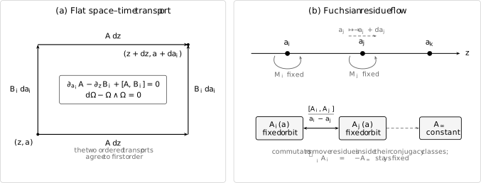
Flat transport makes the $z$-then-$a_i$ and $a_i$-then-$z$ paths agree. Inserting a Fuchsian pole ansatz converts this infinitesimal path independence into pairwise commutator exchange among the residues, while transported monodromy matrices $M_j$ remain fixed.

Zero curvature determines every sign

The $z$–$a_i$ component of flatness is

$$\frac{\partial A}{\partial a_i} - \frac{\partial B_i}{\partial z} + [A,B_i] =0.$$

First isolate the potentially dangerous second-order pole:

$$\frac{\partial}{\partial a_i} \frac{1}{z-a_i} = \frac{1}{(z-a_i)^2}, \qquad \frac{\partial}{\partial z} \left( -\frac{A_i}{z-a_i} \right) = \frac{A_i}{(z-a_i)^2}.$$

Therefore

$$\begin{aligned} \frac{\partial A}{\partial a_i} &= \frac{A_i}{(z-a_i)^2} + \sum_{j=1}^{n} \frac{\partial_{a_i}A_j}{z-a_j}, \\ \frac{\partial B_i}{\partial z} &= \frac{A_i}{(z-a_i)^2}, \\ [A,B_i] &= \sum_{j\ne i} \frac{[A_i,A_j]} {(z-a_i)(z-a_j)}. \end{aligned}$$

The double poles cancel before any evolution equation is used. Had the sign of $B_i$ been positive, they would add instead.

For $i\ne j$, use

$$\frac{1}{(z-a_i)(z-a_j)} = \frac{1}{a_i-a_j} \left( \frac{1}{z-a_i} - \frac{1}{z-a_j} \right).$$

Equating the residue at $z=a_j$ gives the off-diagonal equation

$$\frac{\partial A_j}{\partial a_i} = \frac{[A_i,A_j]}{a_i-a_j}, \qquad i\ne j.$$

Equating the residue at the moving pole $z=a_i$ gives the diagonal equation

$$\frac{\partial A_i}{\partial a_i} = -\sum_{j\ne i} \frac{[A_i,A_j]}{a_i-a_j}.$$

Together these are the Schlesinger equations. Their compact one-form version is

$$\dd A_i = -\sum_{j\ne i} [A_i,A_j]\, \dd\log(a_i-a_j).$$

The compact form makes two structural facts visible. Only relative pole positions occur, and each unordered pair $\{i,j\}$ transfers equal and opposite commutator terms between $A_i$ and $A_j$.

A quick sign audit

For $i\ne j$, interchange $i$ and $j$ in the off-diagonal equation:

$$\partial_{a_j}A_i = \frac{[A_j,A_i]}{a_j-a_i} = \frac{[A_i,A_j]}{a_i-a_j}.$$

The numerator and denominator both change sign. This equality is an easy way to detect a copied convention that does not match the present left-action system.

Multi-time compatibility adds no new equations

Flatness also has an $a_i$–$a_j$ component. In the present convention it is

$$\frac{\partial B_j}{\partial a_i} - \frac{\partial B_i}{\partial a_j} - [B_i,B_j] =0, \qquad i\ne j.$$

Substitute the Schlesinger equations. Since $a_i$ and $a_j$ are independent coordinates,

$$\begin{aligned} \partial_{a_i}B_j-\partial_{a_j}B_i &= \frac{[A_i,A_j]} {(z-a_i)(z-a_j)}, \\ [B_i,B_j] &= \frac{[A_i,A_j]} {(z-a_i)(z-a_j)}. \end{aligned}$$

Thus the time–time curvature vanishes. Conversely, the full Pfaffian system

$$\dd Y = \sum_{i=1}^{n} A_i\,\dd\log(z-a_i)\,Y$$

is Frobenius integrable exactly when the residues obey Schlesinger. On a simply connected domain avoiding both pole collisions and singularities of the residue chart, the value of $Y$ at one point determines a common local solution in all variables.

Flat transport freezes marked monodromy

Choose a base point in the punctured $z$-sphere and transport both it and a system of based loops continuously as $\boldsymbol a$ varies. Let $Y^\gamma$ denote analytic continuation along one such loop and use the book’s right-monodromy convention

$$Y^\gamma=YM_\gamma.$$

Every $B_i=-A_i/(z-a_i)$ is rational and single-valued in $z$. Consequently, analytic continuation commutes with the time equation:

$$\frac{\partial Y^\gamma}{\partial a_i} = B_iY^\gamma.$$

On the other hand, differentiating $Y^\gamma=YM_\gamma$ gives

$$\frac{\partial Y^\gamma}{\partial a_i} = B_iYM_\gamma + Y\frac{\partial M_\gamma}{\partial a_i}.$$

Comparison yields

$$\frac{\partial M_\gamma}{\partial a_i}=0.$$

Thus every based monodromy matrix, not merely its trace, is constant in the time-horizontal frame. The ordered sphere relation

$$M_1M_2\cdots M_nM_\infty=I$$

is preserved with the same order. If one instead changes the base frame by a time-dependent matrix, the tuple undergoes a simultaneous conjugation; the intrinsic statement is constancy of the marked Betti point.

The marking matters globally. Continuing the pole configuration around a nontrivial loop can braid the generators of the punctured sphere. On the universal cover of configuration space the matrices above are constant; after descending, one must include the corresponding pure-braid or Hurwitz action described on the monodromy-moduli page.

Residue orbits and the matrix at infinity are fixed

For every time $a_k$, each residue evolves tangentially to its adjoint orbit. Indeed,

$$\partial_{a_k}A_i=[\Gamma_{ki},A_i],$$

where

$$\Gamma_{ki} = \begin{cases} \displaystyle \frac{A_k}{a_k-a_i}, & k\ne i, \\ \displaystyle \sum_{j\ne i} \frac{A_j}{a_i-a_j}, & k=i. \end{cases}$$

For every positive integer $r$,

$$\begin{aligned} \partial_{a_k}\operatorname{tr}(A_i^r) &= r\operatorname{tr} \left( A_i^{r-1}[\Gamma_{ki},A_i] \right) \\ &=0. \end{aligned}$$

Hence the characteristic polynomial, eigenvalues, and residue conjugacy class are constant. More precisely, integrating $\partial_{a_k}A_i=[\Gamma_{ki},A_i]$ along a local path gives

$$A_i(\boldsymbol a) = G_i(\boldsymbol a) A_i(\boldsymbol a^{(0)}) G_i(\boldsymbol a)^{-1}.$$

Thus the conclusion includes the Jordan type, which traces alone need not determine. In traceless rank two, if

$$\operatorname{spec}A_i = \left\{ \frac{\theta_i}{2}, -\frac{\theta_i}{2} \right\},$$

then

$$\operatorname{tr}(A_i^2) = \frac{\theta_i^2}{2}, \qquad \det A_i = -\frac{\theta_i^2}{4},$$

and $\theta_i$ is fixed, up to the already chosen exponent lift and eigenvalue ordering.

Summing the Schlesinger equations over all finite residues cancels each pairwise contribution:

$$\partial_{a_k} \left( \sum_{i=1}^{n}A_i \right) =0.$$

Therefore

$$\partial_{a_k}A_\infty=0.$$

This is a statement about matrix entries in Schlesinger gauge. In a different time-dependent global frame, $A_\infty$ may be conjugated while its orbit remains fixed.

The pairwise quantities $\operatorname{tr}(A_iA_j)$ are not generally first integrals. They enter the nonautonomous Hamiltonians and usually vary with the pole positions.

This explains a useful terminological distinction. Schlesinger flow is isomonodromic, but it is not an isospectral flow of the pointwise matrix $A(z,\boldsymbol a)$. What is preserved is the monodromy representation and the separate residue spectra, not the eigenvalues of $A$ at a fixed value of $z$.

Affine motions are not true deformation times

There are $n$ finite position variables because infinity has already been distinguished. Two combinations describe changes of affine coordinate rather than motion in the moduli of marked spheres.

For simultaneous translation, the compact Schlesinger form gives

$$\sum_{j=1}^{n} \frac{\partial A_i}{\partial a_j} =0.$$

For simultaneous dilation,

$$\sum_{j=1}^{n} a_j\frac{\partial A_i}{\partial a_j} =[A_i,A_\infty].$$

The right-hand side is a common infinitesimal conjugation, generated by $-A_\infty$, and therefore disappears on the quotient by global gauge. Thus the $n$ finite positions contain

$$n-2=(n+1)-3$$

essential times, agreeing with the dimension $m-3$ of the configuration space when $m=n+1$ counts the pole at infinity.

Four poles leave one essential time

Use a Möbius transformation to place four labeled poles at $0,t,1,\infty$. The coefficient and deformation matrices are

$$\begin{aligned} A(z;t) &= \frac{A_0(t)}{z} + \frac{A_t(t)}{z-t} + \frac{A_1(t)}{z-1}, \\ B_t(z;t) &= -\frac{A_t(t)}{z-t}, \\ A_\infty &= -A_0-A_t-A_1. \end{aligned}$$

Only the cross-ratio $t$ remains after quotienting by Möbius maps. The Schlesinger equations reduce to

$$\begin{aligned} \frac{\dd A_0}{\dd t} &= \frac{[A_t,A_0]}{t}, \\ \frac{\dd A_1}{\dd t} &= \frac{[A_t,A_1]}{t-1}, \\ \frac{\dd A_t}{\dd t} &= -\frac{[A_t,A_0]}{t} - \frac{[A_t,A_1]}{t-1}, \\ \frac{\dd A_\infty}{\dd t} &=0. \end{aligned}$$

For traceless rank two on generic fixed residue orbits, the reduced two-dimensional phase space yields Painlevé VI. The displayed matrix system is not yet the scalar Painlevé equation. Reaching that equation requires symplectic reduction, a choice of Darboux coordinates, and elimination of the momentum; those steps are developed on the later Hamiltonian and Painlevé–Heun pages.

The two fixed singular times $t=0$ and $t=1$ are collisions of the moving pole with $0$ and $1$. A third collision lies at $t=\infty$. These are singularities of the nonautonomous deformation equation and should not be confused with movable poles of a particular solution.

Exact controls: abelian and noncommuting

Exact solutions are valuable because they test the Lax pair, not only the residue ODE. The first control is deliberately degenerate. Let

$$H= \begin{pmatrix} 1&0\\ 0&-1 \end{pmatrix},$$

choose constants $h_0,h_t,h_1$, and set

$$A_0=h_0H, \qquad A_t=h_tH, \qquad A_1=h_1H.$$

All commutators vanish, so every residue is constant. On a declared system of branches,

$$Y(z,t) = z^{h_0H} (z-t)^{h_tH} (z-1)^{h_1H}$$

satisfies

$$\partial_zY=AY, \qquad \partial_tY=-\frac{A_t}{z-t}Y.$$

Its local monodromies

$$M_j=\ee^{2\pi\ii h_jH}$$

are visibly independent of $t$. This is a clean control for signs and branches, but it does not test a commutator term.

A hypergeometric Schlesinger trajectory

For a noncommuting test, introduce

$$E= \begin{pmatrix} 0&1\\ 0&0 \end{pmatrix}, \qquad [H,E]=2E,$$

and use the upper-triangular ansatz

$$A_j=h_jH+b_j(t)E, \qquad j\in\{0,t,1\}.$$

Require the off-diagonal part of $A_\infty$ to vanish:

$$b_0+b_t+b_1=0.$$

Because

$$[A_i,A_j] = 2(h_ib_j-h_jb_i)E,$$

the matrix equations become the linear system

$$\begin{aligned} t\,b_0' &= 2\left[ (h_t+h_0)b_0+h_0b_1 \right], \\ (t-1)b_1' &= 2\left[ h_1b_0+(h_t+h_1)b_1 \right], \\ b_t &= -b_0-b_1. \end{aligned}$$

Assume $h_0\ne0$. Eliminating $b_1$ gives Gauss’s equation

$$t(1-t)b_0'' + \left[ c-(a+b+1)t \right]b_0' - ab\,b_0 =0,$$

with

$$\begin{gathered} a=-2h_t, \qquad b=-2(h_0+h_1+h_t), \\ c=1-2(h_0+h_t). \end{gathered}$$

When $c\notin\{0,-1,-2,\ldots\}$, its standard Frobenius branch at $t=0$ is therefore

$$b_0(t)={}_2F_1(a,b;c;t),$$

and

$$\begin{aligned} b_1(t) &= \frac{ t b_0'(t)-2(h_t+h_0)b_0(t) }{ 2h_0 }, \\ b_t(t) &= -b_0(t)-b_1(t). \end{aligned}$$

Take the rational parameters

$$h_0=\frac17, \qquad h_t=\frac16, \qquad h_1=\frac15.$$

Then

$$\begin{aligned} b_0(t) &= {}_2F_1 \left( -\frac13,-\frac{107}{105}; \frac8{21};t \right), \\ b_1(t) &= \frac72\,t b_0'(t) - \frac{13}{6}b_0(t), \\ b_t(t) &= -b_0(t)-b_1(t), \end{aligned}$$

and

$$\begin{aligned} A_0&=\frac17H+b_0E, & A_t&=\frac16H+b_tE, \\ A_1&=\frac15H+b_1E, & A_\infty&=-\frac{107}{210}H. \end{aligned}$$

The four exponent differences are

$$\frac27, \qquad \frac13, \qquad \frac25, \qquad -\frac{107}{105},$$

so every pole is nonresonant. The family is noncommuting whenever $h_ib_j-h_jb_i\ne0$, yet all residues preserve the line $\mathbb Ce_1$. It is therefore a reducible hypergeometric—or Riccati—locus of the Schlesinger system, not a generic Painlevé VI trajectory.

At $t=1/2$, high-precision evaluation gives

$$\begin{array}{c|r} \text{quantity}&\text{value}\\ \hline b_0& 1.444660071902323853 \\ b_1& -1.578562338666542931 \\ b_t& 0.133902266764219078 \end{array}$$

and

$$\begin{array}{c|r} \text{quantity}&\text{value}\\ \hline b_0'& 0.886591133593424048 \\ b_1'& 1.159496705855737217 \\ b_t'& -2.046087839449161264. \end{array}$$

Substitution into the three scalar equations supplies an independent checkpoint for code. For a meaningful test, compute $b_0'$ from

$$\frac{\dd}{\dd t} {}_2F_1(a,b;c;t) = \frac{ab}{c} {}_2F_1(a+1,b+1;c+1;t)$$

rather than differentiating the first-order Schlesinger right-hand side that is being tested.

The benchmark also warns against false invariants. Here $\operatorname{tr}(A_iA_j)=2h_ih_j$ happens to be constant because products of strictly upper-triangular parts have zero trace. Pairwise residue traces vary for a generic irreducible solution.

Gauge normalization and the converse statement

The formula $B_i=-A_i/(z-a_i)$ is a gauge choice. If

$$Y=G(\boldsymbol a)\widetilde Y$$

with $G$ independent of $z$, then

$$\begin{aligned} \widetilde A &= G^{-1}AG, \\ \widetilde B_i &= G^{-1}B_iG - G^{-1}\partial_{a_i}G. \end{aligned}$$

A general isoprincipal deformation may therefore display

$$B_i = -\frac{A_i}{z-a_i} + K_i(\boldsymbol a).$$

When the time connection $K_i\,\dd a_i$ is flat, a local $z$-independent gauge removes it. Schlesinger gauge is the normalization $K_i=0$; it is also the normalization in which $A_\infty$ is a constant matrix rather than merely moving by conjugation.

The forward implication is unconditional within the Fuchsian chart:

$$\text{Schlesinger} \Longrightarrow \text{constant marked monodromy}.$$

The converse needs local information. An isoprincipal family keeps the full principal factors in its local Levelt factorizations fixed, not only the conjugacy classes of ordinary monodromy. For Fuchsian systems, locally in Schlesinger gauge—or modulo a $z$-independent time gauge—

$$\text{Schlesinger} \ \text{(locally, modulo time gauge)} \Longleftrightarrow \text{isoprincipal} \Longrightarrow \text{isomonodromic}.$$

The first equivalence remains valid in resonance under the standard normalized Fuchsian hypotheses. If every pole, including infinity, is nonresonant, an isomonodromic family is isoprincipal and the three notions coincide locally, up to the time-dependent global gauge just described.

At resonance, constant ordinary monodromy is weaker. A Levelt lattice, logarithmic coefficient, or principal factor can vary without changing the ordinary monodromy tuple. Genuine non-Schlesinger isomonodromic deformations then exist. Fixing exponent eigenvalues alone does not repair the converse; one must fix the appropriate full local principal data.

Two different boundaries of the residue chart

The denominators $a_i-a_j$ expose one boundary immediately, but it is not the only one.

Boundary	What fails	Appropriate response
Pole collision $a_i=a_j$	The point leaves configuration space and Fuchsian singularities merge	Choose a scaled confluence limit; the limiting problem is generally irregular
Malgrange divisor	The poles can remain distinct, but the inverse Riemann–Hilbert family leaves the trivial-bundle chart	Change bundle chart or allow meromorphic residue coordinates

Near a collision, simply substituting $a_i=a_j$ in Schlesinger is meaningless. A controlled limit must specify how positions, residues, and possibly the spectral variable scale; later chapters use precisely such limits to reach confluent Heun and irregular Painlevé systems.

At the second boundary, the abstract isomonodromic family can remain well-defined while the underlying holomorphic bundle changes splitting type. The matrices $A_i(\boldsymbol a)$ in one trivialization may then develop movable poles in time. Under the standard hypotheses, Schlesinger solutions continue meromorphically on the universal cover of configuration space; the polar set of this chart is the Malgrange divisor. The tau function will encode this obstruction on a later page.

Reducible systems introduce a third, milder warning: the differential equations remain valid, but the quotient moduli space can be singular because the stabilizer jumps. The hypergeometric benchmark above lives exactly on such a reducible locus.

Hamiltonian and tau previews

The residue flow has Hamiltonians

$$H_i = \sum_{j\ne i} \frac{\operatorname{tr}(A_iA_j)} {a_i-a_j} = \operatorname*{res}_{z=a_i} \frac12\operatorname{tr}A(z)^2.$$

For the four-pole chart,

$$H_t = \frac{\operatorname{tr}(A_tA_0)}{t} + \frac{\operatorname{tr}(A_tA_1)}{t-1}.$$

The next page derives these formulas from the Kirillov–Kostant form and relates them to accessory parameters. The page after that proves the closedness statement behind $\partial_{a_i}\log\tau=H_i$. Here the formulas serve only as a forward normalization check; neither $H_i$ nor a pairwise residue trace is generally constant.

For the triangular benchmark,

$$H_t = \frac{1}{21t} + \frac{1}{15(t-1)}.$$

This simple expression will let the tau-function page check its signs and branch powers independently.

Common pitfalls

Guessing the sign of the deformation matrix. Different left/right and connection conventions move signs around. Differentiate $(z-a_i)^{-1}$ with respect to both $z$ and $a_i$; cancellation of the double pole fixes the sign in the declared convention.

Writing residue dynamics without a time equation. The matrices $A_i(\boldsymbol a)$ alone do not constitute a Lax pair. Monodromy preservation follows from the single-valued rational matrices $B_i$ and the flat extended connection.

Calling every trace an invariant. The spectral invariants of each individual residue and the matrix $A_\infty$ are preserved in Schlesinger gauge. The cross traces $\operatorname{tr}(A_iA_j)$ generally move.

Equating isomonodromy and Schlesinger at resonance. Constant ordinary monodromy does not fix all resonant Levelt data. The equivalence is with isoprincipal deformation; nonresonance restores the converse from ordinary isomonodromy.

Treating every blow-up as a pole collision. A collision leaves configuration space. A Malgrange pole can occur with all punctures distinct because the chosen trivial-bundle chart fails.

Presenting a reducible exact solution as generic Painlevé VI. The triangular benchmark tests every commutator sign, but its invariant line reduces the nonlinear dynamics to a Gauss equation.

Exercises

1. Recover both Schlesinger equations

Starting from

$$A=\sum_j\frac{A_j}{z-a_j}, \qquad B_i=-\frac{A_i}{z-a_i},$$

derive the $z$–$a_i$ compatibility equation and equate residues at $z=a_i$ and $z=a_j$.

Solution

The double poles cancel because

$$\partial_{a_i}(z-a_i)^{-1} = \partial_z[-(z-a_i)^{-1}] = (z-a_i)^{-2}.$$

The remaining identity is

$$\sum_j \frac{\partial_{a_i}A_j}{z-a_j} + \sum_{j\ne i} \frac{[A_i,A_j]} {(z-a_i)(z-a_j)} =0.$$

Partial fractions give residue $-[A_i,A_j]/(a_i-a_j)$ at $a_j$, hence

$$\partial_{a_i}A_j = \frac{[A_i,A_j]}{a_i-a_j} \quad (j\ne i).$$

The residue at $a_i$ is the sum of the opposite terms, giving

$$\partial_{a_i}A_i = -\sum_{j\ne i} \frac{[A_i,A_j]}{a_i-a_j}.$$

2. Check the time–time curvature

For $i\ne j$, verify directly that

$$\partial_{a_i}B_j - \partial_{a_j}B_i - [B_i,B_j]=0.$$

Solution

The off-diagonal Schlesinger equation gives

$$\begin{aligned} \partial_{a_i}B_j &= -\frac{[A_i,A_j]} {(a_i-a_j)(z-a_j)}, \\ \partial_{a_j}B_i &= -\frac{[A_j,A_i]} {(a_j-a_i)(z-a_i)}. \end{aligned}$$

Combining the two fractions,

$$\partial_{a_i}B_j-\partial_{a_j}B_i = \frac{[A_i,A_j]} {(z-a_i)(z-a_j)} =[B_i,B_j].$$

Moving the final term to the left proves the stated curvature equation.

3. Prove preservation of local spectra

Show that every $\operatorname{tr}(A_i^r)$ is independent of every time and that $A_\infty$ is constant in Schlesinger gauge.

Solution

Each derivative has the form $\partial_{a_k}A_i=[\Gamma_{ki},A_i]$. Cyclicity of trace gives

$$\partial_{a_k}\operatorname{tr}(A_i^r) = r\operatorname{tr} \left( A_i^{r-1}[\Gamma_{ki},A_i] \right) =0.$$

For the sum of finite residues, the contribution associated with every unordered pair $\{i,j\}$ cancels. Hence

$$\partial_{a_k}\sum_iA_i=0,$$

and $A_\infty=-\sum_iA_i$ is constant.

4. Audit the commuting fundamental matrix

Differentiate

$$Y=z^{h_0H}(z-t)^{h_tH}(z-1)^{h_1H}$$

in $z$ and $t$, and compute the three finite local monodromy matrices.

Solution

All factors commute. Logarithmic differentiation in $z$ gives

$$(\partial_zY)Y^{-1} = \frac{h_0H}{z} + \frac{h_tH}{z-t} + \frac{h_1H}{z-1} =A.$$

Only the middle factor depends on $t$, so

$$(\partial_tY)Y^{-1} = -\frac{h_tH}{z-t} = -\frac{A_t}{z-t}.$$

A positive circuit around $a_j$ adds $2\pi\ii$ to $\log(z-a_j)$ and therefore gives

$$M_j=\ee^{2\pi\ii h_jH}.$$

None depends on $t$.

5. Reduce the triangular flow to Gauss’s equation

Starting with $A_j=h_jH+b_jE$, $b_t=-b_0-b_1$, and $h_0\ne0$, derive the two first-order equations for $b_0,b_1$ and eliminate $b_1$.

Solution

Since $[H,E]=2E$,

$$[A_i,A_j] = 2(h_ib_j-h_jb_i)E.$$

Substitution into the $A_0$ and $A_1$ equations gives

$$\begin{aligned} t b_0' &= 2[(h_t+h_0)b_0+h_0b_1], \\ (t-1)b_1' &= 2[h_1b_0+(h_t+h_1)b_1]. \end{aligned}$$

Solve the first equation for $b_1$, differentiate it, and use the second equation to remove $b_1'$:

$$b_1 = \frac{ t b_0'-2(h_t+h_0)b_0 }{ 2h_0 }, \qquad 2h_0b_1' = t b_0'' + [1-2(h_t+h_0)]b_0'.$$

Substitution into the second first-order equation gives the intermediate identity

$$\begin{aligned} (t-1) \left\{ t b_0'' + [1-2(h_t+h_0)]b_0' \right\} ={}& 4h_0h_1b_0 \\ &+ 2(h_t+h_1) \left\{ t b_0' - 2(h_t+h_0)b_0 \right\}. \end{aligned}$$

After collecting terms one obtains

$$t(1-t)b_0'' + [c-(a+b+1)t]b_0' - ab\,b_0 =0,$$

where

$$a=-2h_t, \qquad b=-2(h_0+h_1+h_t), \qquad c=1-2(h_0+h_t).$$

6. Locate what is special about the benchmark

For the rational triangular example, verify nonresonance, reducibility, and the constancy of $\operatorname{tr}(A_iA_j)$. Explain why the last property is not a general Schlesinger invariant.

Solution

The eigenvalues of $h_iH+b_iE$ are $\pm h_i$, so the finite exponent differences are $2/7$, $1/3$, and $2/5$. At infinity the difference is $-107/105$. None is an integer, hence all four poles are nonresonant.

Every upper-triangular residue preserves $\mathbb Ce_1$, so the representation is reducible. Moreover, $E^2=0$ and both $HE$ and $EH$ have zero trace. Therefore

$$\operatorname{tr}(A_iA_j)=2h_ih_j,$$

which is constant. A generic residue tuple is not simultaneously triangular, and its cross traces enter explicitly time-dependent Hamiltonians; the Schlesinger equations do not set their derivatives to zero.

7. Remove the affine coordinate directions

Use the compact Schlesinger form to prove

$$\sum_j\partial_{a_j}A_i=0, \qquad \sum_j a_j\partial_{a_j}A_i=[A_i,A_\infty].$$

Why do these identities leave $n-2$ essential times when there are $n$ finite poles?

Solution

For simultaneous translation, set every $\dd a_j=\dd c$. Then $\dd\log(a_i-a_j)=0$, so $\dd A_i=0$ and

$$\sum_j\partial_{a_j}A_i=0.$$

For simultaneous dilation, set $\dd a_j=a_j\,\dd s$. Every logarithmic difference changes by $\dd s$, hence

$$\begin{aligned} \frac{\dd A_i}{\dd s} &= -\sum_{j\ne i}[A_i,A_j] \\ &= -\left[ A_i,-A_\infty-A_i \right] =[A_i,A_\infty]. \end{aligned}$$

This is common conjugation by the generator $-A_\infty$ and vanishes on the global-gauge quotient. Translation and dilation remove two of the $n$ finite position directions, leaving $n-2$ true times.

8. Distinguish two singular limits

Suppose a four-pole solution becomes singular at $t=t_*$. What observations distinguish a pole collision from a Malgrange-chart failure?

Solution

If $t_*\in\{0,1,\infty\}$, the marked configuration reaches its boundary: two punctures collide after the chosen normalization. A meaningful limit requires a confluence scaling and generally produces an irregular singularity.

If $t_*\notin\{0,1,\infty\}$ while the residue matrices acquire a pole, all punctures remain distinct. The likely failure is the chosen global trivialization: the inverse Riemann–Hilbert bundle has changed splitting type, placing the deformation on the Malgrange divisor. One should change bundle chart rather than merge singularities.

References

• L. Schlesinger, “Über eine Klasse von Differentialsystemen beliebiger Ordnung mit festen kritischen Punkten”, Journal für die reine und angewandte Mathematik 141 (1912), 96–145. The original source of the deformation equations.
• K. Iwasaki, H. Kimura, S. Shimomura, and M. Yoshida, From Gauss to Painlevé: A Modern Theory of Special Functions, Vieweg, 1991. A reader-facing bridge from classical Fuchsian equations to monodromy-preserving deformation.
• M. Jimbo, T. Miwa, and K. Ueno, “Monodromy Preserving Deformation of Linear Ordinary Differential Equations with Rational Coefficients. I. General Theory and τ-Function”, Physica D 2 (1981), 306–352. The modern rational-connection formulation and its regular and irregular extensions.
• V. Katsnelson and D. Volok, “Deformations of Fuchsian Systems of Linear Differential Equations and the Schlesinger System”, Mathematical Physics, Analysis and Geometry 9 (2006), 135–186. A precise treatment of isoprincipal deformations and the resonant converse problem.
• Y. Bibilo and G. Filipuk, “Non-Schlesinger Isomonodromic Deformations of Fuchsian Systems and Middle Convolution”, Symmetry, Integrability and Geometry: Methods and Applications 11 (2015), 023. Explicit resonant non-Schlesinger deformations.
• B. Malgrange, “Déformations isomonodromiques des singularités régulières”, RCP 25 31 (1983), 1–26. Global continuation and the bundle-theoretic obstruction behind the Malgrange divisor.
• T. Miwa, “Painlevé Property of Monodromy Preserving Deformation Equations and the Analyticity of Tau Functions”, Publications of the Research Institute for Mathematical Sciences 17 (1981), 703–721. Meromorphic continuation and the Painlevé property for the normalized monodromy-preserving deformation equations treated there.