BPZ Equations as Second-Order Linear ODEs

The level-two null relation guarantees a differential operator of second order in the degenerate coordinate. Whether that operator is an ODE is decided only after the three global Ward identities have been used and the true moduli have been counted. This page performs that reduction in the two configurations that recur throughout the book.

With three nondegenerate primaries and one degenerate field, the sphere has one cross-ratio. The BPZ constraint closes to a rigid ODE with three regular singularities, and a scalar gauge turns it into the Gauss hypergeometric equation. With four nondegenerate primaries and an additional degenerate probe, two variables survive. The exact finite-central-charge equation retains a modulus derivative and is a PDE. Only after a controlled heavy–light factorization does its leading part become the four-pole oper underlying a Heun equation.

Keep the three stages separate

1. Null-vector decoupling gives an exact configuration-space PDE.
2. Global Ward identities and position fixing give either a hypergeometric ODE or a two-variable PDE.
3. A heavy–light asymptotic ansatz can turn the latter PDE into a Heun oper.

The second and third arrows are additional operations, not consequences of the Kac label alone.

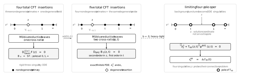
The number of total CFT insertions and the number of singularities of the limiting ODE are different counts. Four total insertions leave one cross-ratio and a rigid Gauss ODE; five leave the exact $(z,t)$ BPZ PDE, which becomes a four-pole oper only after the stated heavy–light factorization.

Position fixing comes after the global Ward identities

For the $(2,1)$ field, the previous page derived

$$\left[ b^{-2}\partial_z^2 + \sum_i \left( \frac{\Delta_i^{\mathrm{CFT}}}{(z-z_i)^2} + \frac{1}{z-z_i}\partial_{z_i} \right) \right]\mathscr B = 0.$$

Three global Ward identities eliminate the derivatives associated with translations, dilations, and special conformal transformations. The safe order of operations is:

Step	Operation	Datum that must be retained
1	Keep all insertions finite	Every $\partial_{z_i}$ term
2	Solve the three global Ward identities	All conformal-weight terms
3	Send three positions to $0$, $1$, and $\infty$	The normalized definition of the field at infinity
4	Choose branches and a scalar prefactor	Unit-leading local bases

Setting $z_i=0,1,\infty$ before eliminating the associated derivatives loses weight-dependent terms. In particular, a derivative does not vanish merely because its coordinate will later be fixed.

For a primary at infinity, use

$$V_\infty(\infty) := \lim_{R\to\infty} R^{2\Delta_\infty^{\mathrm{CFT}}} V_\infty(R)$$

only after the finite-$R$ Ward reduction.

To see what this warning protects, begin with the unspecialized block

$$\widehat{\mathscr B} \left( z;x_0,x_1,x_R \right) := \left\langle V_\infty(x_R) V_1(x_1) V_{-b/2}(z) V_0(x_0) \right\rangle_{\mathrm{ch}},$$

then evaluate it at three finite ordinary positions:

$$\mathscr B_R(z) := \widehat{\mathscr B}(z;0,1,R).$$

Let $\partial_0$, $\partial_1$, and $\partial_R$ denote the corresponding derivatives of $\widehat{\mathscr B}$, evaluated only after differentiation. Define the three operators

$$\begin{aligned} \mathcal W_0 &= \partial_z, \\ \mathcal W_1 &= z\partial_z+\Sigma_\Delta, \\ \mathcal W_2 &= z^2\partial_z +2z\Delta_{\mathrm d} +2\Delta_1^{\mathrm{CFT}} +2R\Delta_\infty^{\mathrm{CFT}}, \end{aligned}$$

where

$$\Sigma_\Delta = \Delta_0^{\mathrm{CFT}} +\Delta_1^{\mathrm{CFT}} +\Delta_\infty^{\mathrm{CFT}} +\Delta_{\mathrm d}.$$

At $x_0=0$, $x_1=1$, and $x_R=R$, the global Ward identities become

$$\begin{pmatrix} 1&1&1\\ 0&1&R\\ 0&1&R^2 \end{pmatrix} \begin{pmatrix} \partial_0\\ \partial_1\\ \partial_R \end{pmatrix} \mathscr B_R = - \begin{pmatrix} \mathcal W_0\\ \mathcal W_1\\ \mathcal W_2 \end{pmatrix} \mathscr B_R.$$

The inverse system is short enough to keep in the normalization ledger:

$$\begin{aligned} \partial_0\mathscr B_R &= \left[ -\mathcal W_0 +\frac{R+1}{R}\mathcal W_1 -\frac1R\mathcal W_2 \right]\mathscr B_R, \\ \partial_1\mathscr B_R &= \frac{ \mathcal W_2-R\mathcal W_1 }{R-1} \mathscr B_R, \\ \partial_R\mathscr B_R &= \frac{ \mathcal W_1-\mathcal W_2 }{R(R-1)} \mathscr B_R. \end{aligned}$$

Substitute these expressions into the universal BPZ constraint, and only then take

$$\mathscr B_4(z) = \lim_{R\to\infty} R^{2\Delta_\infty^{\mathrm{CFT}}} \mathscr B_R(z).$$

The terms proportional to $\Delta_\infty^{\mathrm{CFT}}$ survive this limit. They are precisely the terms that a premature substitution $R=\infty$ would hide.

Four total insertions give the hypergeometric ODE

Consider the chiral object

$$\mathscr B_4(z) := \left\langle V_\infty(\infty) V_1(1) V_{-b/2}(z) V_0(0) \right\rangle_{\mathrm{ch}}.$$

Write

$$\Delta_{\mathrm d} := \Delta_{2,1}^{\mathrm{CFT}} = -\frac12-\frac{3b^2}{4}.$$

Applying the global reduction gives

$$\begin{aligned} 0 ={}& b^{-2}\mathscr B_4'' - \left( \frac1z+\frac{1}{z-1} \right)\mathscr B_4' \\ &+ \left[ \frac{\Delta_0^{\mathrm{CFT}}}{z^2} + \frac{\Delta_1^{\mathrm{CFT}}}{(z-1)^2} \right]\mathscr B_4 \\ &+ \frac{ \Delta_\infty^{\mathrm{CFT}} - \Delta_0^{\mathrm{CFT}} - \Delta_1^{\mathrm{CFT}} - \Delta_{\mathrm d} }{ z(z-1) } \mathscr B_4. \end{aligned}$$

The only singular points are $0$, $1$, and $\infty$, and all are regular. There is no accessory parameter: a second-order Fuchsian equation on the sphere with three singular points is rigid.

The local exponents retain the two fusion channels

Use the centered momenta

$$a_{\mathrm L,i} = \alpha_i-\frac{Q_{\mathrm L}}2, \qquad i\in\{0,1,\infty\}.$$

At a finite insertion, define

$$\rho_{i,\epsilon_{\mathrm f}} := \frac{bQ_{\mathrm L}}2 + \epsilon_{\mathrm f} b\,a_{\mathrm L,i}, \qquad \epsilon_{\mathrm f}=\pm1.$$

The local behaviors of $\mathscr B_4$ are

Point	Local coordinate	Exponents
$0$	$z$	$\rho_{0,+},\ \rho_{0,-}$
$1$	$1-z$	$\rho_{1,+},\ \rho_{1,-}$
$\infty$	$w=1/z$	$\nu_{\infty,+},\ \nu_{\infty,-}$

Here the infinity convention is $\mathscr B_4(z)\sim z^{-\nu_{\infty,\epsilon_{\mathrm f}}}$, with

$$\nu_{\infty,\epsilon_{\mathrm f}} = 2\Delta_{\mathrm d} + \frac{bQ_{\mathrm L}}2 + \epsilon_{\mathrm f}b\,a_{\mathrm L,\infty} = -\frac12-b^2 + \epsilon_{\mathrm f}b\,a_{\mathrm L,\infty}.$$

The shift by $2\Delta_{\mathrm d}$ comes from moving the degenerate field through the coordinate inversion used to define the insertion at infinity. The exponent sums obey the Fuchs relation

$$\left( \rho_{0,+}+\rho_{0,-} \right) + \left( \rho_{1,+}+\rho_{1,-} \right) + \left( \nu_{\infty,+}+\nu_{\infty,-} \right) = 1.$$

A scalar gauge exposes the Gauss equation

Choose branches of $\Log z$ and $\Log(1-z)$ that are real on $0<z<1$, and set

$$\mathscr B_4(z) = S(z)F(z), \qquad S(z) = z^{\rho_{0,+}} (1-z)^{\rho_{1,+}}.$$

The selected prefactor extracts one fusion exponent at $0$ and one at $1$. Substitution into the BPZ ODE gives

$$z(1-z)F'' + \left[ C-(A+B+1)z \right]F' - ABF = 0,$$

where

$$\begin{aligned} A &= \frac12 + b \left( a_{\mathrm L,0} + a_{\mathrm L,1} - a_{\mathrm L,\infty} \right), \\ B &= \frac12 + b \left( a_{\mathrm L,0} + a_{\mathrm L,1} + a_{\mathrm L,\infty} \right), \\ C &= 1+2b\,a_{\mathrm L,0}. \end{aligned}$$

This is exactly the convention used in the hypergeometric connection benchmark, with its parameters $(a,b,c)$ replaced by $(A,B,C)$ so that the Liouville coupling $b$ is not overloaded.

The oriented exponent differences translate as

$$\begin{aligned} 1-C &= -2b\,a_{\mathrm L,0}, \\ C-A-B &= -2b\,a_{\mathrm L,1}, \\ A-B &= -2b\,a_{\mathrm L,\infty}. \end{aligned}$$

Thus Kac fusion data determine all three exponent differences of the rigid ODE.

Both branches form one unit-leading basis

For generic nonresonant parameters, the unit-leading Gauss basis at zero is the basis whose coefficient multiplying each selected Frobenius power is one:

$$\begin{aligned} f_0(z) &= {}_2F_1(A,B;C;z), \\ g_0(z) &= z^{1-C} {}_2F_1 \left( A-C+1, B-C+1; 2-C; z \right). \end{aligned}$$

Multiplying both columns by the same scalar gauge gives

$$\Phi_0^{\mathrm{BPZ}} = S(z) \left( f_0(z), g_0(z) \right).$$

The first column behaves as $z^{\rho_{0,+}}$ and carries intermediate momentum $\alpha_0-b/2$. Since

$$\rho_{0,+}+1-C = \rho_{0,-},$$

the second behaves as $z^{\rho_{0,-}}$ and carries $\alpha_0+b/2$. The two local fusion channels are therefore the two Frobenius columns of one second-order equation.

Because $S(z)$ has unit leading coefficient at both $0$ and $1$ on the chosen cut, the zero-to-one gamma connection matrix from Chapter 2 applies directly to these unit-leading BPZ bases. At infinity, the phase of $(1-z)^{\rho_{1,+}}$ must be included in the normalization ledger. Degenerate fusion and braiding normalizations are the subject of the next page.

Resonant basis limits

The displayed bases assume

$$C\notin\mathbb Z, \qquad C-A-B\notin\mathbb Z.$$

A diagonal basis at infinity additionally assumes $A-B\notin\mathbb Z$. At resonance the differential equation remains well defined, but a unit-leading power basis must be replaced by a logarithmic or limiting basis before connection coefficients are evaluated.

Five total insertions leave an exact modulus derivative

Now add a fourth nondegenerate primary at $t$:

$$\mathscr B_5(z,t) := \left\langle V_\infty(\infty) V_1(1) V_t(t) V_{-b/2}(z) V_0(0) \right\rangle_{\mathrm{ch}}.$$

After the same global Ward reduction, the exact equation is

$$\begin{aligned} 0 ={}& \bigg[ b^{-2}\partial_z^2 - \left( \frac1z+\frac{1}{z-1} \right)\partial_z \\ &\quad+ \frac{ t(t-1) }{ z(z-1)(z-t) } \partial_t \\ &\quad+ \frac{\Delta_0^{\mathrm{CFT}}}{z^2} + \frac{\Delta_t^{\mathrm{CFT}}}{(z-t)^2} + \frac{\Delta_1^{\mathrm{CFT}}}{(z-1)^2} \\ &\quad+ \frac{ \Delta_\infty^{\mathrm{CFT}} - \Delta_0^{\mathrm{CFT}} - \Delta_t^{\mathrm{CFT}} - \Delta_1^{\mathrm{CFT}} - \Delta_{\mathrm d} }{ z(z-1) } \bigg] \mathscr B_5. \end{aligned}$$

The coefficient of $\partial_t$ can also be obtained by combining the two terms

$$\frac{t}{z(z-t)}\partial_t - \frac{t}{z(z-1)}\partial_t.$$

It is nonzero for generic $t$. Freezing the numerical value of $t$ does not set the derivative of the block with respect to $t$ to zero. The finite-$b$ equation is a two-variable BPZ PDE, sometimes called a nonstationary Heun equation; it is not the ordinary general Heun ODE.

The singular divisors in the probe coordinate are

$$z=0, \qquad z=t, \qquad z=1, \qquad z=\infty.$$

Their local fusion exponents are still determined by $\alpha_i\mapsto\alpha_i\pm b/2$. What is missing at finite $b$ is a $z$-independent replacement for the modulus derivative.

The Heun oper is a conditional leading equation

The later heavy–light analysis will justify the scaling

$$\Delta_i^{\mathrm{CFT}} = \frac{\delta_i}{b^2}+O(1), \qquad i\in\{0,t,1,\infty\},$$

The selected background channel is scaled simultaneously:

$$\Delta_{0t}^{\mathrm{CFT}} = \frac{\delta_{0t}}{b^2}+O(1).$$

Its parameter enters $f_{0t}$ even though it appears in $T_{\mathrm{op}}$ only through $c_t^{\mathrm{op}}$. The corresponding factorization is

$$\mathscr B_5(z,t) \sim \exp \left( \frac{f_{0t}(t)}{b^2} \right) \left[ \psi^{\mathrm{BPZ}}(z;t)+O(b^2) \right].$$

Here $f_{0t}(t)$ is the leading classical four-point block in the chosen background channel, while $\psi^{\mathrm{BPZ}}$ is the light probe factor. For the moment, treat this as a conditional asymptotic ansatz. Then

$$b^2\partial_t\mathscr B_5 \sim \exp \left( \frac{f_{0t}}{b^2} \right) \left[ \partial_t f_{0t}\, \psi^{\mathrm{BPZ}} + O(b^2) \right].$$

Multiplying the exact PDE by $b^2$ and taking its leading term suppresses the first $z$-derivative and the residual $\partial_t\psi^{\mathrm{BPZ}}$. One obtains

$$\left[ \partial_z^2 + T_{\mathrm{op}}(z;t) \right] \psi^{\mathrm{BPZ}}(z;t) = 0,$$

with

$$\begin{aligned} T_{\mathrm{op}}(z;t) ={}& \frac{\delta_0}{z^2} + \frac{\delta_t}{(z-t)^2} + \frac{\delta_1}{(z-1)^2} \\ &+ \frac{ \delta_\infty-\delta_0-\delta_t-\delta_1 }{ z(z-1) } \\ &+ \frac{ t(t-1)c_t^{\mathrm{op}} }{ z(z-1)(z-t) }. \end{aligned}$$

For the full block normalization written above,

$$c_t^{\mathrm{op}} = \partial_t f_{0t}.$$

Removing an OPE prefactor shifts this relation by the derivative of that prefactor. Thus $c_t^{\mathrm{op}}$ is the fixed-coordinate four-pole oper residue in the declared $0,t,1,\infty$ coordinate, not yet the accessory parameter of a chosen standard general Heun equation. Page 5 will justify the heavy–light factorization; page 6 will fix the normalization ledger and the complete accessory crosswalk.

Common pitfalls

Fixing coordinates before reducing derivatives. The global Ward identities turn the derivatives of the fixed insertions into weight and probe-derivative terms. Setting them to zero first gives the wrong ODE.

Calling the five-insertion equation a finite-$b$ Heun ODE. Its $\partial_t$ term is exact. A Heun oper appears only after the declared heavy–light factorization or another legitimate elimination of the modulus dynamics.

Forgetting the scalar gauge. Hypergeometric functions solve the equation for $F$, not the ungauged block $\mathscr B_4$. The powers in $S(z)$ carry the physical fusion exponents and their branches.

Reusing the symbol $b$ for a Gauss parameter. Here $b$ is the Liouville coupling. The Gauss parameters are $(A,B,C)$, while the lowercase $(a,b,c)$ notation appears only in the linked benchmark.

Equating accessory normalizations. The oper residue, the derivative of a normalized classical block, and the standard Heun parameter differ by explicit gauge and OPE-prefactor shifts. The later accessory page will compare them only after every prefactor has been declared.

Exercises

1. Complete the finite-position Ward reduction

Invert the finite-$R$ Ward system and recover the three derivative formulas in the text. Substitute them into the universal BPZ constraint before taking the normalized limit $R\to\infty$.

Solution

Subtracting the second Ward equation from the third gives

$$R(R-1)\partial_R\mathscr B_R = \left( \mathcal W_1-\mathcal W_2 \right)\mathscr B_R.$$

Back-substitution into the second and first rows then gives

$$\begin{aligned} \partial_1\mathscr B_R &= \frac{ \mathcal W_2-R\mathcal W_1 }{R-1} \mathscr B_R, \\ \partial_0\mathscr B_R &= \left[ -\mathcal W_0 +\frac{R+1}{R}\mathcal W_1 -\frac1R\mathcal W_2 \right]\mathscr B_R. \end{aligned}$$

Together with the expression for $\partial_R\mathscr B_R$, these remove all three ordinary-coordinate derivatives. Substitution followed by

$$\mathscr B_4(z) = \lim_{R\to\infty} R^{2\Delta_\infty^{\mathrm{CFT}}} \mathscr B_R(z)$$

yields

$$\begin{aligned} 0 ={}& \bigg[ b^{-2}\partial_z^2 - \left( \frac1z+\frac1{z-1} \right)\partial_z \\ &+ \frac{\Delta_0^{\mathrm{CFT}}}{z^2} + \frac{\Delta_1^{\mathrm{CFT}}}{(z-1)^2} \\ &+ \frac{ \Delta_\infty^{\mathrm{CFT}} -\Delta_0^{\mathrm{CFT}} -\Delta_1^{\mathrm{CFT}} -\Delta_{\mathrm d} }{ z(z-1) } \bigg]\mathscr B_4. \end{aligned}$$

The $2R\Delta_\infty^{\mathrm{CFT}}$ term in $\mathcal W_2$ is why the infinity weight remains after the normalized limit.

2. Check the infinity exponent pair

Insert $\mathscr B_4(z)\sim z^{-\nu}$ into the four-insertion BPZ ODE. Recover $\nu_{\infty,\pm}$ and verify the Fuchs sum.

Solution

At large $z$, the potential coefficient is $(\Delta_\infty^{\mathrm{CFT}}-\Delta_{\mathrm d})/z^2$. The leading equation is

$$b^{-2}\nu(\nu+1) + 2\nu + \Delta_\infty^{\mathrm{CFT}} - \Delta_{\mathrm d} = 0.$$

Using $\Delta_\infty^{\mathrm{CFT}} =Q_{\mathrm L}^2/4-a_{\mathrm L,\infty}^2$ gives

$$\nu_{\infty,\pm} = -\frac12-b^2 \pm b\,a_{\mathrm L,\infty}.$$

The finite-point exponent sums are each $1+b^2$, while the infinity sum is $-1-2b^2$. Their total is one.

3. Derive the Gauss parameters

Substitute $\mathscr B_4=z^{\rho_{0,+}}(1-z)^{\rho_{1,+}}F$ into the BPZ ODE and show that the double poles cancel.

Solution

The double pole at zero cancels because

$$b^{-2}\rho_{0,+}(\rho_{0,+}-1) - \rho_{0,+} + \Delta_0^{\mathrm{CFT}} = 0,$$

and the same indicial identity holds at one. Collecting the remaining simple-pole and regular terms yields

$$z(1-z)F'' + \left[ C-(A+B+1)z \right]F' - ABF = 0$$

with

$$\begin{aligned} C &= 2\rho_{0,+}-b^2, \\ A+B+1-C &= 2\rho_{1,+}-b^2, \\ AB &= \left[ \frac12 +b \left( a_{\mathrm L,0}+a_{\mathrm L,1} \right) \right]^2 - b^2a_{\mathrm L,\infty}^2. \end{aligned}$$

Using $bQ_{\mathrm L}=1+b^2$ in the first two lines and factoring the third recovers the displayed $A$, $B$, and $C$.

4. Identify both fusion branches

Show that the second Gauss solution at zero carries the exponent $\rho_{0,-}$ and rewrite its parameters using $a_{\mathrm L,0}\mapsto-a_{\mathrm L,0}$.

Solution

Since $1-C=-2b\,a_{\mathrm L,0}$,

$$\rho_{0,+}+1-C = \frac{bQ_{\mathrm L}}2 - b\,a_{\mathrm L,0} = \rho_{0,-}.$$

Moreover,

$$\begin{aligned} A-C+1 &= \frac12 + b \left( -a_{\mathrm L,0} + a_{\mathrm L,1} - a_{\mathrm L,\infty} \right), \\ B-C+1 &= \frac12 + b \left( -a_{\mathrm L,0} + a_{\mathrm L,1} + a_{\mathrm L,\infty} \right), \\ 2-C &= 1-2b\,a_{\mathrm L,0}. \end{aligned}$$

These are the same parameter formulas with the opposite fusion sign at zero.

5. Simplify the modulus derivative

Verify that the two $\partial_t$ terms in the expanded five-insertion equation combine into the coefficient used in the text.

Solution

One has

$$\begin{aligned} \frac{t}{z(z-t)} - \frac{t}{z(z-1)} &= \frac{ t\left[(z-1)-(z-t)\right] }{ z(z-1)(z-t) } \\ &= \frac{t(t-1)}{z(z-1)(z-t)}. \end{aligned}$$

The coefficient vanishes only at a boundary degeneration $t\in\{0,1\}$, where the insertion configuration itself becomes singular.

6. Derive the Gauss Wronskian

Use Abel’s identity to determine the Wronskian of two independent Gauss solutions. What changes when an exponent difference is integral?

Solution

After division by $z(1-z)$, the coefficient of $F'$ is

$$P(z) = \frac{C}{z} + \frac{C-A-B-1}{1-z}.$$

Abel’s identity, $W_F'=-P W_F$, therefore gives

$$W_F(z) = K z^{-C} (1-z)^{C-A-B-1}, \qquad K\neq0.$$

An integral exponent difference does not invalidate Abel’s identity or the differential equation. It invalidates the generic diagonal power-basis formula: the second local column must instead be reconstructed by a resonant Frobenius calculation, which determines whether a logarithm occurs, or by a controlled parameter limit.

7. Recover the Gauss coefficient recurrence

Let $F(z)=\sum_{n\geq0}f_nz^n$ with $f_0=1$. Derive the coefficient recurrence and state when the series terminates.

Solution

$$(n+1)(n+C)f_{n+1} = (n+A)(n+B)f_n, \qquad n\geq0.$$

Hence

$$\frac{f_{n+1}}{f_n} = \frac{(n+A)(n+B)}{(n+1)(n+C)}.$$

If $A=-N$ or $B=-N$ for an integer $N\geq0$, the numerator vanishes at $n=N$, and a unit-leading polynomial branch exists provided $n+C\neq0$ for $0\leq n\leq N$. If a denominator vanishes in that range, use the resonant or limiting recurrence and impose polynomial termination separately. If a resonant denominator occurs only after termination, choose the newly free coefficient to be zero to retain the polynomial branch.

References

• A. A. Belavin, A. M. Polyakov, and A. B. Zamolodchikov, “Infinite Conformal Symmetry in Two-Dimensional Quantum Field Theory”, Nuclear Physics B 241 (1984), 333–380. Null-vector differential equations and degenerate four-point blocks.
• S. Ribault, Conformal Field Theory on the Plane, 2014. Fixed-position BPZ equations, degenerate fusion exponents, and hypergeometric solutions.
• G. Bonelli, C. Iossa, D. Panea Lichtig, and A. Tanzini, “Irregular Liouville Correlators and Connection Formulae for Heun Functions”, Communications in Mathematical Physics 397 (2023), 635–727. Exact four- and five-insertion BPZ equations, centered-momentum solutions, and controlled classical reductions.
• A. Litvinov, S. Lukyanov, N. Nekrasov, and A. Zamolodchikov, “Classical Conformal Blocks and Painlevé VI”, Journal of High Energy Physics 2014 (7), 144. Classical-block exponentiation, monodromy data, and accessory parameters.
• NIST Digital Library of Mathematical Functions, §15.10, Hypergeometric Differential Equation. Canonical local solutions, exponent data, and analytic continuation conventions.