Skip to content

Painlevé Lax Systems and Heun Reductions

A four-pole rank-two Fuchsian system and the general Heun equation are closely related, but they are not the same object at a generic isomonodromic time. Cyclic reduction of the matrix system introduces a fifth, apparent scalar singularity. Its position moves according to Painlevé VI. A genuine four-singularity Heun equation appears only on a specified collision slice, after an integer shift of the exponent lifts and a declared scalar gauge.

In the normalization developed below, the result is particularly useful. Let t0t_0 be the fourth Heun singularity, let αHβH\alpha_{\mathrm H}\beta_{\mathrm H} be the product of its two exponents at infinity, and let τJ(ρ;t)\tau_{\mathrm J}(\rho;t) be the traceless JMU tau function for the shifted Painlevé data ρ\rho. If θt=ϑt1\theta_t=\vartheta_t-1 is the Painlevé exponent at the collision pole, then

qH=t0αHβH+t0(t01)[ ⁣d ⁣dtlogτJ(ρ;t)θ0θt2tθ1θt2(t1)]t=t0,\begin{aligned} q_{\mathrm H} ={}& t_0\alpha_{\mathrm H}\beta_{\mathrm H} \\ &+ t_0(t_0-1) \left. \left[ \frac{\dd}{\dd t}\log\tau_{\mathrm J}(\rho;t) - \frac{\theta_0\theta_t}{2t} - \frac{\theta_1\theta_t}{2(t-1)} \right] \right|_{t=t_0}, \end{aligned}

provided the accompanying collision constraint is satisfied. That constraint may be written as a derivative condition, or as a zero of a Schlesinger-transformed tau function. Neither statement says that an arbitrary Heun equation is “equal to Painlevé VI,” and neither makes a tau zero a spectral condition without further boundary data.

Several nearby quantities have similar names. This ledger fixes their use on this page.

SymbolRole
ttIsomonodromic time and one true moving pole
(q,p)(q,p)Spectral Darboux coordinates in the traceless gauge of the preceding pages; qq is an apparent-pole position
(λ,μ)(\lambda,\mu)Polynomial coordinates in the rank-one residue gauge used for the collision calculation; exactly λ=q\lambda=q and μ=P\mu=P
KVIK_{\mathrm{VI}}One polynomial Painlevé VI Hamiltonian; it differs from the bare JMU Hamiltonian by time-dependent canonical terms
K0K_0Compact Heun accessory in the collision gauge below
qHq_{\mathrm H}The standard Heun accessory in the house convention of Chapter 3
τJ\tau_{\mathrm J}JMU tau function of the traceless residue system, so tlogτJ=Ht\partial_t\log\tau_{\mathrm J}=H_t
τρ+\tau_{\rho^+}A neighboring tau function obtained by one elementary Schlesinger transformation

In particular, the apparent coordinate qq is never the standard Heun accessory qHq_{\mathrm H}.

Start from the normalized traceless system

Φz=(A0z+Atzt+A1z1)Φ,A=A0AtA1,\frac{\partial\Phi}{\partial z} = \left( \frac{A_0}{z} + \frac{A_t}{z-t} + \frac{A_1}{z-1} \right)\Phi, \qquad A_\infty=-A_0-A_t-A_1,

with

specAν={θν2,θν2}.\operatorname{spec}A_\nu = \left\{ \frac{\theta_\nu}{2}, - \frac{\theta_\nu}{2} \right\}.

After diagonalizing AA_\infty, the upper-right entry has the form

b(z)=χ(zq)z(z1)(zt),χ0.b(z) = \frac{\chi(z-q)} {z(z-1)(z-t)}, \qquad \chi\ne0.

Eliminating the second component and applying the Liouville gauge gives

ψ(z)+Tdef(z)ψ(z)=0.\psi''(z)+T_{\mathrm{def}}(z)\psi(z)=0.

Its finite-pole structure is

Tdef(z)=s{0,t,1}[1θs24(zs)2+cszs]34(zq)2+cqzq.\begin{aligned} T_{\mathrm{def}}(z) ={}& \sum_{s\in\{0,t,1\}} \left[ \frac{1-\theta_s^2}{4(z-s)^2} + \frac{c_s}{z-s} \right] \\ &- \frac{3}{4(z-q)^2} + \frac{c_q}{z-q}. \end{aligned}

The first three points are true singularities. At z=qz=q, the local exponents are 1/2-1/2 and 3/23/2, so their difference is 22. The coefficient

cq=p+12(1q+1qt+1q1)c_q = p + \frac12 \left( \frac1q + \frac1{q-t} + \frac1{q-1} \right)

and define dqd_q by

Tdef(z)=34(zq)2+cqzq+dq+O(zq).T_{\mathrm{def}}(z) = -\frac{3}{4(z-q)^2} + \frac{c_q}{z-q} + d_q + O(z-q).

The no-log relation is

dq=cq2.d_q=-c_q^2.

Before the Liouville gauge, the apparent exponents are 0,20,2 and the local monodromy is II. In the displayed normal form the square-root gauge changes it to the central matrix I-I. It remains projectively trivial, so qq is not a fifth point of the matrix connection.

Expansion at infinity supplies two linear constraints,

c0+ct+c1+cq=0,c_0+c_t+c_1+c_q=0,

and

1θ24=s{0,t,1}1θs2434+tct+c1+qcq.\begin{aligned} \frac{1-\theta_\infty^2}{4} ={}& \sum_{s\in\{0,t,1\}} \frac{1-\theta_s^2}{4} - \frac34 \\ &+ t\,c_t+c_1+q\,c_q. \end{aligned}

Together with the no-log condition, these leave one scalar accessory in addition to the apparent position. This is the scalar image of the two-dimensional four-pole phase space.

Use the shifted momentum from the preceding page,

P=p+12[θ0q+θ1q1+θtqt].P = p + \frac12 \left[ \frac{\theta_0}{q} + \frac{\theta_1}{q-1} + \frac{\theta_t}{q-t} \right].

One standard polynomial Hamiltonian is

t(t1)KVI=q(q1)(qt)P2[θ0(q1)(qt)+θ1q(qt)+(θt1)q(q1)]P+κ(qt),\begin{aligned} t(t-1)K_{\mathrm{VI}} ={}& q(q-1)(q-t)P^2 \\ &- \Bigl[ \theta_0(q-1)(q-t) + \theta_1q(q-t) \\ &\hspace{3.2em} + (\theta_t-1)q(q-1) \Bigr]P \\ &+ \kappa(q-t), \end{aligned}

where

κ=(θ0+θ1+θt1)2(θ1)24.\kappa = \frac{ (\theta_0+\theta_1+\theta_t-1)^2 - (\theta_\infty-1)^2 }{4}.

The first Hamilton equation gives

2q(q1)(qt)P=t(t1)q+θ0(q1)(qt)+θ1q(qt)+(θt1)q(q1).\begin{aligned} 2q(q-1)(q-t)P ={}& t(t-1)q' \\ &+ \theta_0(q-1)(q-t) + \theta_1q(q-t) \\ &+ (\theta_t-1)q(q-1). \end{aligned}

Substituting this expression into the second Hamilton equation and simplifying yields

q=12(1q+1q1+1qt)(q)2(1t+1t1+1qt)q+q(q1)(qt)2t2(t1)2[(θ1)2θ02tq2+θ12(t1)(q1)2+(1θt2)t(t1)(qt)2].\begin{aligned} q'' ={}& \frac12 \left( \frac1q+\frac1{q-1}+\frac1{q-t} \right)(q')^2 \\ &- \left( \frac1t+\frac1{t-1}+\frac1{q-t} \right)q' \\ &+ \frac{q(q-1)(q-t)} {2t^2(t-1)^2} \Biggl[ (\theta_\infty-1)^2 - \frac{\theta_0^2t}{q^2} \\ &\hspace{7.0em} + \frac{\theta_1^2(t-1)}{(q-1)^2} + \frac{(1-\theta_t^2)t(t-1)} {(q-t)^2} \Biggr]. \end{aligned}

This is Painlevé VI in the parameter convention

(αVI,βVI,γVI,δVI)=12((θ1)2,θ02,θ12,1θt2).\left( \alpha_{\mathrm{VI}}, \beta_{\mathrm{VI}}, \gamma_{\mathrm{VI}}, \delta_{\mathrm{VI}} \right) = \frac12 \left( (\theta_\infty-1)^2, - \theta_0^2, \theta_1^2, 1-\theta_t^2 \right).

The nonlinear function q(t)q(t) is the apparent singularity of the scalar Lax equation. The fixed singular times of Painlevé VI are 0,1,0,1,\infty. The value q=tq=t makes the displayed second-order equation look singular because eliminating momentum divided by qtq-t. In the original spectral chart pp generally diverges there, but the shifted polynomial momentum PP remains finite and resolves the collision branch. Adjacent Okamoto charts cover the complementary branch and exceptional parameter loci.

The displayed KVIK_{\mathrm{VI}} generates the chosen (q,P)(q,P) chart. It is not automatically the bare JMU derivative HtH_t. Their exact relation contains the canonical and gauge shifts derived on the preceding two pages.

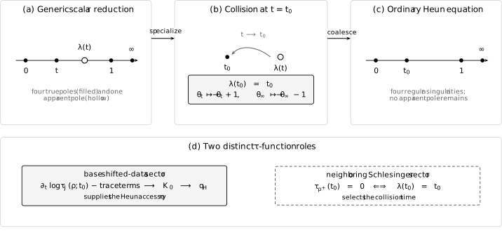
From a four-pole Lax system through Painlevé VI to a Heun collision slice

A generic cyclic reduction has one moving apparent point λ\lambda and is governed by Painlevé VI. On the marked slice λ(t0)=t0\lambda(t_0)=t_0, an integer exponent shift and a scalar gauge merge that point with the true pole, leaving a four-singularity Heun equation. The standard accessory qHq_{\mathrm H} is reconstructed from the shifted-data JMU logarithmic derivative after trace corrections; the neighboring tau zero selects the collision time.

A collision slice produces the Heun equation

Section titled “A collision slice produces the Heun equation”

The collision algebra is clearest in a second, explicitly declared gauge. Up to this point the traceless residues were denoted by AνA_\nu. In this section only, rename that connection B(z)B(z) and reserve A(z)A(z) for its rank-one scalar lift:

A(z)=B(z)+12(θ0z+θtzt+θ1z1)I.A(z) = B(z) + \frac12 \left( \frac{\theta_0}{z} + \frac{\theta_t}{z-t} + \frac{\theta_1}{z-1} \right)I.

Each finite residue now has eigenvalues 0,θν0,\theta_\nu rather than ±θν/2\pm\theta_\nu/2. Choose

A=diag(κ,κ+),κ±=12(θ0+θt+θ1±θ).A_\infty = \operatorname{diag}(\kappa_-,\kappa_+), \qquad \kappa_\pm = - \frac12 \left( \theta_0+\theta_t+\theta_1 \pm\theta_\infty \right).

This adds scalar multiples of the identity to the traceless residues. It preserves the projective monodromy but changes the chosen exponent lifts and multiplies tau by an elementary factor.

Write the zero of A12(z)A_{12}(z) as λ\lambda, and define μ=A11(λ)\mu=A_{11}(\lambda). The scalar lift leaves the upper-right entry unchanged and gives

λ=q,μ=p+12(θ0q+θtqt+θ1q1)=P.\lambda=q, \qquad \mu = p + \frac12 \left( \frac{\theta_0}{q} + \frac{\theta_t}{q-t} + \frac{\theta_1}{q-1} \right) =P.

Thus the Hamiltonian K\mathcal K below is the same polynomial KVIK_{\mathrm{VI}} written in (λ,μ)(\lambda,\mu) coordinates, since

κ(1+κ+)=κ.\kappa_-(1+\kappa_+)=\kappa.

The first component obeys

y+(1θ0z+1θtzt+1θ1z11zλ)y+[κ(1+κ+)z(z1)t(t1)Kz(zt)(z1)+λ(λ1)μz(zλ)(z1)]y=0.\begin{aligned} y'' &+ \left( \frac{1-\theta_0}{z} + \frac{1-\theta_t}{z-t} + \frac{1-\theta_1}{z-1} - \frac1{z-\lambda} \right)y' \\ &+ \Biggl[ \frac{\kappa_-(1+\kappa_+)} {z(z-1)} - \frac{t(t-1)\mathcal K} {z(z-t)(z-1)} \\ &\hspace{5.4em} + \frac{\lambda(\lambda-1)\mu} {z(z-\lambda)(z-1)} \Biggr]y =0. \end{aligned}

Apparency at λ\lambda fixes the Hamiltonian

K(λ,μ,t)=λ(λt)(λ1)t(t1)[μ2(θ0λ+θ1λ1+θt1λt)μ+κ(1+κ+)λ(λ1)].\begin{aligned} \mathcal K(\lambda,\mu,t) ={}& \frac{\lambda(\lambda-t)(\lambda-1)} {t(t-1)} \Biggl[ \mu^2 \\ &- \left( \frac{\theta_0}{\lambda} + \frac{\theta_1}{\lambda-1} + \frac{\theta_t-1}{\lambda-t} \right)\mu \\ &+ \frac{\kappa_-(1+\kappa_+)} {\lambda(\lambda-1)} \Biggr]. \end{aligned}

At an ordinary point t0{0,1}t_0\notin\{0,1\}, impose

λ(t0)=t0,μ(t0)=K0θt,θt0.\lambda(t_0)=t_0, \qquad \mu(t_0)=-\frac{K_0}{\theta_t}, \qquad \theta_t\ne0.

Although the printed Hamiltonian appears singular at λ=t\lambda=t, its limit is finite:

K(t0)=(θt1)μ(t0).\mathcal K(t_0) = - (\theta_t-1)\mu(t_0).

The two scalar accessory terms then combine because

μ(t0)K(t0)=θtμ(t0)=K0.\mu(t_0)-\mathcal K(t_0) = \theta_t\mu(t_0) = -K_0.

At the same time, the coefficient of yy' at the merged point becomes θt/(zt0)-\theta_t/(z-t_0). Introduce the Heun exponent differences

ϑ0=θ0,ϑt=θt+1,ϑ1=θ1,ϑ=θ1.\begin{aligned} \vartheta_0&=\theta_0, & \vartheta_t&=\theta_t+1, \\ \vartheta_1&=\theta_1, & \vartheta_\infty&=\theta_\infty-1. \end{aligned}

The collision equation is

y+(1ϑ0z+1ϑ1z1+1ϑtzt0)y+[αHβHz(z1)t0(t01)K0z(z1)(zt0)]y=0,\begin{aligned} y'' &+ \left( \frac{1-\vartheta_0}{z} + \frac{1-\vartheta_1}{z-1} + \frac{1-\vartheta_t}{z-t_0} \right)y' \\ &+ \left[ \frac{\alpha_{\mathrm H}\beta_{\mathrm H}} {z(z-1)} - \frac{t_0(t_0-1)K_0} {z(z-1)(z-t_0)} \right]y =0, \end{aligned}

where

αH=1ϑ0+ϑt+ϑ1ϑ2,βH=1ϑ0+ϑt+ϑ1+ϑ2.\begin{aligned} \alpha_{\mathrm H} &= 1- \frac{ \vartheta_0+\vartheta_t+\vartheta_1-\vartheta_\infty }{2}, \\ \beta_{\mathrm H} &= 1- \frac{ \vartheta_0+\vartheta_t+\vartheta_1+\vartheta_\infty }{2}. \end{aligned}

Indeed,

αH=κ,βH=1+κ+,αHβH=ϑ,\alpha_{\mathrm H}=\kappa_-, \qquad \beta_{\mathrm H}=1+\kappa_+, \qquad \alpha_{\mathrm H}-\beta_{\mathrm H} = \vartheta_\infty,

and

αHβH=κ(1+κ+),\alpha_{\mathrm H}\beta_{\mathrm H} = \kappa_-(1+\kappa_+),

and the Fuchs relation is automatic. In the house convention

γH=1ϑ0,δH=1ϑ1,ϵH=1ϑt,aH=t0.\begin{aligned} \gamma_{\mathrm H}&=1-\vartheta_0, & \delta_{\mathrm H}&=1-\vartheta_1, \\ \epsilon_{\mathrm H}&=1-\vartheta_t, & a_{\mathrm H}&=t_0. \end{aligned}

Combining the two fractions in the coefficient of yy finally gives the standard Heun accessory

qH=t0αHβH+t0(t01)K0.q_{\mathrm H} = t_0\alpha_{\mathrm H}\beta_{\mathrm H} + t_0(t_0-1)K_0.

The additive first term is essential. The compact coefficient K0K_0, the normal-form residue ct0c_{t_0}, and the standard parameter qHq_{\mathrm H} are affine coordinates on the same one-dimensional accessory fiber, but they are not numerically identical.

For the Chapter 3 normal form, define

Δνsc=1ϑν24,Λsc=ΔscΔ0scΔ1scΔtsc.\Delta_\nu^{\mathrm{sc}} = \frac{1-\vartheta_\nu^2}{4}, \qquad \Lambda_{\mathrm{sc}} = \Delta_\infty^{\mathrm{sc}} - \Delta_0^{\mathrm{sc}} - \Delta_1^{\mathrm{sc}} - \Delta_t^{\mathrm{sc}}.

Then the remaining two changes of accessory coordinate are

κH=qHγH2(t0δH+ϵH),ct0sc=t0ΛscκHt0(t01).\begin{aligned} \kappa_{\mathrm H} &= q_{\mathrm H} - \frac{\gamma_{\mathrm H}}2 \left( t_0\delta_{\mathrm H} + \epsilon_{\mathrm H} \right), \\ c_{t_0}^{\mathrm{sc}} &= \frac{ t_0\Lambda_{\mathrm{sc}}-\kappa_{\mathrm H} }{ t_0(t_0-1) }. \end{aligned}

Tau constraints separate two neighboring systems

Section titled “Tau constraints separate two neighboring systems”

Write ςij\varsigma_{ij} for the chosen target-Heun composite-monodromy lifts and σij\sigma_{ij} for their shifted Painlevé counterparts. The exponent and composite-monodromy lifts of the deformation system are shifted from the target Heun lifts:

θ0θtθ1θσ0tσ1tσ01ρHϑ0ϑtϑ1ϑς0tς1tς01ρϑ0ϑt1ϑ1ϑ+1ς0t1ς1t1ς01\begin{array}{c|cccc|ccc} &\theta_0&\theta_t&\theta_1&\theta_\infty &\sigma_{0t}&\sigma_{1t}&\sigma_{01} \\ \hline \rho_{\mathrm H} &\vartheta_0&\vartheta_t&\vartheta_1&\vartheta_\infty &\varsigma_{0t}&\varsigma_{1t}&\varsigma_{01} \\ \rho &\vartheta_0&\vartheta_t-1&\vartheta_1&\vartheta_\infty+1 &\varsigma_{0t}-1&\varsigma_{1t}-1&\varsigma_{01} \end{array}

These integer shifts are part of an elementary Schlesinger transformation. Omitting them changes the marked scalar equation even when some projective monodromy invariants look unchanged.

Let

Bν=Aνθν2IB_\nu = A_\nu-\frac{\theta_\nu}{2}I

be the traceless residues, and let τJ(ρ;t)\tau_{\mathrm J}(\rho;t) be their JMU tau function. In the convention fixed on the preceding page,

Ht=tr(BtB0)t+tr(BtB1)t1= ⁣d ⁣dtlogτJ(ρ;t).\begin{aligned} H_t &= \frac{\operatorname{tr}(B_tB_0)}{t} + \frac{\operatorname{tr}(B_tB_1)}{t-1} \\ &= \frac{\dd}{\dd t}\log\tau_{\mathrm J}(\rho;t). \end{aligned}

Passing from the rank-one residues AνA_\nu to BνB_\nu is not invisible:

tr(BtBj)=tr(AtAj)θtθj2,j{0,1}.\operatorname{tr}(B_tB_j) = \operatorname{tr}(A_tA_j) - \frac{\theta_t\theta_j}{2}, \qquad j\in\{0,1\}.

Taking the smooth finite-μ\mu collision limit gives

Ht(t0)=K0+θ0θt2t0+θ1θt2(t01).\begin{aligned} H_t(t_0) ={}& K_0 + \frac{\theta_0\theta_t}{2t_0} + \frac{\theta_1\theta_t}{2(t_0-1)}. \end{aligned}

Therefore the compact accessory is

K0=[ ⁣d ⁣dtlogτJ(ρ;t)θ0θt2tθ1θt2(t1)]t=t0,K_0 = \left. \left[ \frac{\dd}{\dd t}\log\tau_{\mathrm J}(\rho;t) - \frac{\theta_0\theta_t}{2t} - \frac{\theta_1\theta_t}{2(t-1)} \right] \right|_{t=t_0},

and the standard Heun accessory is

qH=t0αHβH+t0(t01) ⁣d ⁣dtlogτJ(ρ;t)t=t0(t01)θ0θt2t0θ1θt2.\begin{aligned} q_{\mathrm H} ={}& t_0\alpha_{\mathrm H}\beta_{\mathrm H} + t_0(t_0-1) \left. \frac{\dd}{\dd t} \log\tau_{\mathrm J}(\rho;t) \right|_{t=t_0} \\ &- \frac{(t_0-1)\theta_0\theta_t}{2} - \frac{t_0\theta_1\theta_t}{2}. \end{aligned}

Combining this expression with the Chapter 3 normal-form dictionary causes all dependence on ϑ0\vartheta_0, ϑ1\vartheta_1, and ϑ\vartheta_\infty outside the tau derivative to cancel:

ct0sc= ⁣d ⁣dtlogτJ(ρ;t)t=t0+(ϑt1)(2t01)2t0(t01).c_{t_0}^{\mathrm{sc}} = - \left. \frac{\dd}{\dd t} \log\tau_{\mathrm J}(\rho;t) \right|_{t=t_0} + \frac{ (\vartheta_t-1)(2t_0-1) }{ 2t_0(t_0-1) }.

This compact identity belongs to the displayed cyclic component, infinity eigenline ordering, and collision branch. Another component or the other collision branch has a correspondingly shifted formula.

Set

ζJ(t)=t(t1) ⁣d ⁣dtlogτJ(ρ;t).\zeta_{\mathrm J}(t) = t(t-1) \frac{\dd}{\dd t} \log\tau_{\mathrm J}(\rho;t).

The two collision data for this traceless JMU representative are

ζJ(t0)=t0(t01)K0+(t01)θ0θt2+t0θ1θt2,ζJ(t0)=θt(θθt)2.\begin{aligned} \zeta_{\mathrm J}(t_0) ={}& t_0(t_0-1)K_0 \\ &+ \frac{(t_0-1)\theta_0\theta_t}{2} + \frac{t_0\theta_1\theta_t}{2}, \\ \zeta_{\mathrm J}'(t_0) ={}& \frac{\theta_t(\theta_\infty-\theta_t)}{2}. \end{aligned}

For the second line, the finite-μ\mu branch makes BtB_t triangular with diagonal entries θt/2,θt/2-\theta_t/2,\theta_t/2. Since B0+B1=BBtB_0+B_1=-B_\infty-B_t, taking the trace of Bt(B0+B1)B_t(B_0+B_1) gives the displayed derivative without choosing residue coordinates.

The scalar lift instead has the tau representative

τA(t)=tθ0θt/2(t1)θtθ1/2τJ(ρ;t)\tau_A(t) = t^{\theta_0\theta_t/2} (t-1)^{\theta_t\theta_1/2} \tau_{\mathrm J}(\rho;t)

on a chosen logarithm branch. Its sigma variable is shifted by the exact affine function

ζA(t)=t(t1) ⁣d ⁣dtlogτA(t)=ζJ(t)+(t1)θ0θt2+tθtθ12.\begin{aligned} \zeta_A(t) &= t(t-1)\frac{\dd}{\dd t}\log\tau_A(t) \\ &= \zeta_{\mathrm J}(t) + \frac{(t-1)\theta_0\theta_t}{2} + \frac{t\theta_t\theta_1}{2}. \end{aligned}

This time-dependent factor is a change of tau representative induced by the scalar gauge. It is not the time-independent JMU normalization constant. All accessory formulas on this page use τJ(ρ;t)\tau_{\mathrm J}(\rho;t) and ζJ\zeta_{\mathrm J}.

The neighboring tau zero selects the collision

Section titled “The neighboring tau zero selects the collision”

Let ρ+\rho^+ be obtained from ρ\rho by

(θt,θ,σ0t,σ1t)(θt+1,θ1,σ0t+1,σ1t+1).(\theta_t,\theta_\infty,\sigma_{0t},\sigma_{1t}) \longmapsto (\theta_t+1,\theta_\infty-1,\sigma_{0t}+1,\sigma_{1t}+1).

Let ρ\rho^- denote the inverse shift, and write τρ±\tau_{\rho^\pm} for the corresponding neighboring JMU tau functions. Thus ρ+=ρH\rho^+=\rho_{\mathrm H} in the displayed lift table. On the nonresonant Schlesinger patch, coherent normalizations of the three neighboring tau functions obey the Toda identity

ζJ(t)θt(θθt)2=Cτρ+(t)τρ(t)τJ(ρ;t)2,\begin{aligned} \zeta_{\mathrm J}'(t) - \frac{\theta_t(\theta_\infty-\theta_t)}{2} &= C\, \frac{ \tau_{\rho^+}(t)\tau_{\rho^-}(t) }{ \tau_{\mathrm J}(\rho;t)^2 }, \end{aligned}

where CC is a nonzero, tt-independent normalization constant. At the collision the left-hand side vanishes. Provided the base tau is nonzero, one neighboring factor must vanish; choosing the ++ factor selects λ(t0)=t0\lambda(t_0)=t_0. Thus

τρ+(t0)=0.\tau_{\rho^+}(t_0)=0.

This is the collision branch of the standard Toda identity, equation (3.15) of Anselmo et al. Consequently, the zero of τρ+\tau_{\rho^+} locates the Heun slice, whereas the logarithmic derivative of the generally nonzero τJ(ρ;t)\tau_{\mathrm J}(\rho;t) supplies its accessory. These are two different tau functions.

Choose the target Heun exponent differences

(ϑ0,ϑt,ϑ1,ϑ)=(13,12,14,25)\left( \vartheta_0,\vartheta_t,\vartheta_1,\vartheta_\infty \right) = \left( \frac13,\frac12,\frac14,\frac25 \right)

and set t0=2t_0=2. The shifted Painlevé data are

(θ0,θt,θ1,θ)=(13,12,14,75).\left( \theta_0,\theta_t,\theta_1,\theta_\infty \right) = \left( \frac13,-\frac12,\frac14,\frac75 \right).

Then

κ=79120,1+κ+=31120,\kappa_-=\frac{79}{120}, \qquad 1+\kappa_+=\frac{31}{120},

so

αH=79120,βH=31120,αHβH=244914400.\alpha_{\mathrm H}=\frac{79}{120}, \qquad \beta_{\mathrm H}=\frac{31}{120}, \qquad \alpha_{\mathrm H}\beta_{\mathrm H} = \frac{2449}{14400}.

Take

K0=13,λ(t0)=t0,μ(t0)=23.K_0=\frac13, \qquad \lambda(t_0)=t_0, \qquad \mu(t_0)=\frac23.

Because θt=1/2\theta_t=-1/2, the collision relation μ=K0/θt\mu=-K_0/\theta_t holds. Moreover,

K(t0)=(θt1)μ=1,μK=13=K0.\mathcal K(t_0) = - (\theta_t-1)\mu = 1, \qquad \mu-\mathcal K=-\frac13=-K_0.

The resulting house-convention Heun equation is

y+(23z+34(z1)+12(z2))y+244914400z72497200z(z1)(z2)y=0.\begin{aligned} y'' &+ \left( \frac{2}{3z} + \frac{3}{4(z-1)} + \frac{1}{2(z-2)} \right)y' \\ &+ \frac{ \dfrac{2449}{14400}z - \dfrac{7249}{7200} }{ z(z-1)(z-2) }y =0. \end{aligned}

Indeed,

qH=2(244914400)+2(13)=72497200,q_{\mathrm H} = 2\left(\frac{2449}{14400}\right) + 2\left(\frac13\right) = \frac{7249}{7200},

and

γH+δH+ϵH=2312=αH+βH+1.\gamma_{\mathrm H}+\delta_{\mathrm H}+\epsilon_{\mathrm H} = \frac{23}{12} = \alpha_{\mathrm H}+\beta_{\mathrm H}+1.

The two trace corrections give

Ht(t0)=K0+θ0θt2t0+θ1θt2(t01)=13124116=1148.\begin{aligned} H_t(t_0) &= K_0 + \frac{\theta_0\theta_t}{2t_0} + \frac{\theta_1\theta_t}{2(t_0-1)} \\ &= \frac13-\frac1{24}-\frac1{16} = \frac{11}{48}. \end{aligned}

Hence the traceless JMU sigma data are

ζJ(t0)=1124,ζJ(t0)=1940.\zeta_{\mathrm J}(t_0)=\frac{11}{24}, \qquad \zeta_{\mathrm J}'(t_0)=-\frac{19}{40}.

Conversely, the corrected tau formula gives

qH=24497200+1124+112+18=72497200.\begin{aligned} q_{\mathrm H} ={}& \frac{2449}{7200} + \frac{11}{24} + \frac1{12} + \frac18 \\ &= \frac{7249}{7200}. \end{aligned}

The two Chapter 3 normal-form coordinates are

κH=24497200,ct0sc=2948.\kappa_{\mathrm H} = \frac{2449}{7200}, \qquad c_{t_0}^{\mathrm{sc}} = -\frac{29}{48}.

This benchmark checks the exponent shifts, collision sign, trace corrections, sigma derivative, standard Heun accessory, and normal-form residue with exact arithmetic.

What the reduction does and does not claim

Section titled “What the reduction does and does not claim”

Generic time versus Heun slice. A generic PVI Lax scalarization has an apparent fifth point. HeunG is obtained only on a collision slice or an equivalent specialization in another chart.

Local existence versus a global collision. Prescribing λ(t0)=t0\lambda(t_0)=t_0 and μ(t0)\mu(t_0) gives a local PVI solution away from exceptional parameters. For one fixed global monodromy point, collision times are discrete and need not occur in a chosen domain.

Gauge-specific formula versus invariant content. The printed KVI=KK_{\mathrm{VI}}=\mathcal K, K0K_0, ct0scc_{t_0}^{\mathrm{sc}}, and qHq_{\mathrm H} are different Hamiltonian or scalar coordinates. The monodromy representation is the invariant object; coefficient identities must carry their gauge dictionaries.

Tau zero versus spectral zero. The transformed tau zero enforces the apparent-pole collision. It becomes an eigenvalue or resonance condition only after separate physical boundary constraints are encoded in the monodromy data.

Calling the apparent coordinate the Heun accessory. The PVI dependent variable is q(t)q(t) or λ(t)\lambda(t). The standard Heun accessory is qHq_{\mathrm H} and is obtained only after specialization and an affine translation.

Dropping the integer exponent shifts. The collision changes θt\theta_t by +1+1 and θ\theta_\infty by 1-1 on the Heun side, together with the marked composite lifts. Reusing the unshifted tuple gives the wrong scalar equation.

Using the polynomial Hamiltonian as a tau derivative. The displayed KVIK_{\mathrm{VI}} belongs to a time-dependent Darboux chart. The JMU identity uses the bare residue Hamiltonian HtH_t.

Dropping the trace corrections. The scalar lift and the traceless JMU system have residue Hamiltonians differing by two explicit half-trace terms. They cannot be absorbed into the time-independent multiplicative normalization of tau.

Setting the wrong tau function to zero. The collision uses a Schlesinger-transformed neighbor τρ+\tau_{\rho^+}, while the accessory uses the logarithmic derivative of τJ(ρ;t)\tau_{\mathrm J}(\rho;t). Conflating them produces a spurious pole.

Treating λ=t\lambda=t as a true-pole collision. The true pole remains at t0{0,1}t_0\notin\{0,1\}. It is the apparent point that meets it, so the event is an accessible divisor resolved by the finite-μ\mu chart, not a degeneration of the four-punctured sphere.

Use the rank-one scalar equation to compute the indicial roots at z=λz=\lambda. Why is an additional no-log condition still required?

Solution

Put x=zλx=z-\lambda. The coefficient of yy' is x1+O(1)-x^{-1}+O(1), while the coefficient of yy has at most a simple pole. The indicial polynomial is therefore

ρ(ρ1)ρ=ρ(ρ2),\rho(\rho-1)-\rho = \rho(\rho-2),

with roots 00 and 22. Their integer separation permits a logarithm in the smaller-exponent solution. Expanding that solution in a Taylor series gives one resonant compatibility condition. The printed formula for K(λ,μ,t)\mathcal K(\lambda,\mu,t) is precisely the global coefficient relation that enforces it.

Solve the first Hamilton equation for PP and identify the four standard Painlevé VI parameters after eliminating it.

Solution

Differentiation of KVIK_{\mathrm{VI}} with respect to PP gives

P=12q(q1)(qt)[t(t1)q+θ0(q1)(qt)+θ1q(qt)+(θt1)q(q1)].\begin{aligned} P = \frac{1}{2q(q-1)(q-t)} \Bigl[ &t(t-1)q' \\ &+ \theta_0(q-1)(q-t) \\ &+ \theta_1q(q-t) \\ &+ (\theta_t-1)q(q-1) \Bigr]. \end{aligned}

Substitution into P=qKVIP'=-\partial_qK_{\mathrm{VI}} gives the equation in the body. Comparison with the standard four-parameter form yields

αVI=(θ1)22,βVI=θ022,\alpha_{\mathrm{VI}} = \frac{(\theta_\infty-1)^2}{2}, \quad \beta_{\mathrm{VI}} = -\frac{\theta_0^2}{2},

and

γVI=θ122,δVI=1θt22.\gamma_{\mathrm{VI}} = \frac{\theta_1^2}{2}, \quad \delta_{\mathrm{VI}} = \frac{1-\theta_t^2}{2}.

Take λt0\lambda\to t_0 in K\mathcal K and show that the two scalar accessory terms reduce to t0(t01)K0-t_0(t_0-1)K_0 over the Heun denominator.

Solution

Only the term containing (θt1)μ/(λt)(\theta_t-1)\mu/(\lambda-t) survives the prefactor λ(λt)(λ1)/[t(t1)]\lambda(\lambda-t)(\lambda-1)/[t(t-1)]. Hence

K(t0)=(θt1)μ(t0).\mathcal K(t_0) = -(\theta_t-1)\mu(t_0).

After setting μ(t0)=K0/θt\mu(t_0)=-K_0/\theta_t,

μ(t0)K(t0)=θtμ(t0)=K0.\mu(t_0)-\mathcal K(t_0) = \theta_t\mu(t_0) = -K_0.

The two last terms of the scalar equation therefore combine into

t0(t01)K0z(z1)(zt0).- \frac{t_0(t_0-1)K_0} {z(z-1)(z-t_0)}.

Combine the two fractions in the collision equation and derive the standard Heun parameter qHq_{\mathrm H}.

Solution

With D(z)=z(z1)(zt0)D(z)=z(z-1)(z-t_0),

αHβHz(z1)t0(t01)K0D(z)=αHβH(zt0)t0(t01)K0D(z).\begin{aligned} \frac{\alpha_{\mathrm H}\beta_{\mathrm H}}{z(z-1)} &- \frac{t_0(t_0-1)K_0}{D(z)} \\ &= \frac{ \alpha_{\mathrm H}\beta_{\mathrm H}(z-t_0) - t_0(t_0-1)K_0 }{D(z)}. \end{aligned}

Comparison with (αHβHzqH)/D(z)(\alpha_{\mathrm H}\beta_{\mathrm H}z-q_{\mathrm H})/D(z) gives

qH=t0αHβH+t0(t01)K0.q_{\mathrm H} = t_0\alpha_{\mathrm H}\beta_{\mathrm H} + t_0(t_0-1)K_0.

Starting from the definition of ζJ\zeta_{\mathrm J} and its first collision datum, derive the JMU expression for K0K_0. Then compute the affine change from ζJ\zeta_{\mathrm J} to ζA\zeta_A.

Solution

By definition,

ζJ=t(t1)Ht.\zeta_{\mathrm J} = t(t-1)H_t.

The first collision condition therefore gives

K0=Ht(t0)θ0θt2t0θ1θt2(t01)=[ ⁣d ⁣dtlogτJ(ρ;t)θ0θt2tθ1θt2(t1)]t=t0.\begin{aligned} K_0 ={}& H_t(t_0) - \frac{\theta_0\theta_t}{2t_0} - \frac{\theta_1\theta_t}{2(t_0-1)} \\ &= \left. \left[ \frac{\dd}{\dd t}\log\tau_{\mathrm J}(\rho;t) - \frac{\theta_0\theta_t}{2t} - \frac{\theta_1\theta_t}{2(t-1)} \right] \right|_{t=t_0}. \end{aligned}

Multiplication by the scalar-gauge factor changes the sigma variable by

ζAζJ=(t1)θ0θt2+tθtθ12.\zeta_A-\zeta_{\mathrm J} = \frac{(t-1)\theta_0\theta_t}{2} + \frac{t\theta_t\theta_1}{2}.

The second collision datum itself remains ζJ(t0)=θt(θθt)/2\zeta_{\mathrm J}'(t_0) =\theta_t(\theta_\infty-\theta_t)/2 in the declared traceless representative.

Verify the Fuchs relation, Ht(t0)H_t(t_0), qHq_{\mathrm H}, ζJ(t0)\zeta_{\mathrm J}'(t_0), and ct0scc_{t_0}^{\mathrm{sc}} for the exact example.

Solution

The finite Heun residues are

γH=23,δH=34,ϵH=12.\gamma_{\mathrm H}=\frac23, \qquad \delta_{\mathrm H}=\frac34, \qquad \epsilon_{\mathrm H}=\frac12.

Thus

γH+δH+ϵH=2312.\gamma_{\mathrm H}+\delta_{\mathrm H}+\epsilon_{\mathrm H} = \frac{23}{12}.

Also

αH+βH+1=31+79120+1=2312.\alpha_{\mathrm H}+\beta_{\mathrm H}+1 = \frac{31+79}{120}+1 = \frac{23}{12}.

The JMU derivative is

Ht(t0)=13124116=1148,H_t(t_0) = \frac13-\frac1{24}-\frac1{16} = \frac{11}{48},

so ζJ(t0)=2Ht(t0)=11/24\zeta_{\mathrm J}(t_0)=2H_t(t_0)=11/24. The standard accessory follows either from K0K_0 or from the corrected tau formula:

qH=24497200+1124+112+18=72497200.\begin{aligned} q_{\mathrm H} &= \frac{2449}{7200} + \frac{11}{24} + \frac1{12} + \frac18 \\ &= \frac{7249}{7200}. \end{aligned}

The derivative condition gives

ζJ(t0)=12(75+12)(12)=1940.\begin{aligned} \zeta_{\mathrm J}'(t_0) &= \frac12 \left( \frac75+\frac12 \right) \left( -\frac12 \right) = -\frac{19}{40}. \end{aligned}

Finally, the compact normal-form identity yields

ct0sc=114838=2948.c_{t_0}^{\mathrm{sc}} = -\frac{11}{48} - \frac38 = -\frac{29}{48}.

7. Diagnose a proposed Heun–Painlevé identity

Section titled “7. Diagnose a proposed Heun–Painlevé identity”

A formula sets λ=qH\lambda=q_{\mathrm H} for every tt and evaluates an unshifted tau function at the same data. Identify at least four missing or incorrect steps.

Solution

The proposal:

  1. confuses the apparent position λ(t)\lambda(t) with the standard Heun accessory qHq_{\mathrm H};
  2. ignores that the generic scalar equation has five singularities;
  3. omits the collision condition λ(t0)=t0\lambda(t_0)=t_0;
  4. omits the integer shifts at tt and infinity, and the corresponding composite-lift shifts;
  5. fails to distinguish the original JMU tau function from its Schlesinger-transformed neighbor;
  6. misses the affine term t0αHβHt_0\alpha_{\mathrm H}\beta_{\mathrm H} in the standard accessory.

Any spectral interpretation would additionally require boundary conditions and a spectral-parameter dictionary.