Appendix B: Complex Analysis and Asymptotics

Complex analysis turns local formulae into global data, while asymptotic analysis turns exact objects into controlled approximations. Both operations are convention-sensitive. A logarithm without a sheet, a saddle contribution without an oriented contour, or a period without a lifted cycle is not yet a reproducible quantity.

This appendix is a working desk for the recurring ingredients used throughout the book. It supplies the shortest safe derivations and points to the chapters where the analytic hypotheses are developed in depth.

The six-entry asymptotic passport

Record the analytic domain or covering surface, the base germ and continuation path, all logarithm and square-root branches, the oriented contour or homology class, the large-parameter sector or Borel ray, and the status of the remainder estimate. These six entries separate an identity from a formal expansion and a formal expansion from a summed analytic statement.

Analytic continuation remembers a path

A holomorphic germ $[f]_{z_*}$ can be continued along a path $\gamma:[0,1]\to X$ by a chain of overlapping analytic elements. The endpoint germ can depend on the homotopy class of $\gamma$ in $X$. The monodromy theorem guarantees path independence when the relevant domain is simply connected and continuation exists along every path under consideration. Simple connectivity is sufficient, not necessary: a function can have trivial monodromy on a multiply connected domain.

The house default for elementary powers is

$$-\pi<\operatorname{Arg}z\leq\pi, \qquad \operatorname{Log}z = \log|z|+\ii\operatorname{Arg}z.$$

After continuation around a closed path avoiding the origin,

$$\operatorname{Log}^{\gamma}z = \operatorname{Log}z +2\pi\ii\,\operatorname{wind}(\gamma,0).$$

Consequently,

$$\left(z^\alpha\right)^\gamma = \ee^{ 2\pi\ii\alpha\, \operatorname{wind}(\gamma,0) } z^\alpha.$$

The upper and lower boundary values on the principal cut are, for $x>0$,

$$\operatorname{Log}(-x\pm\ii0) = \log x\pm\pi\ii.$$

Thus $\sqrt z=\exp[\operatorname{Log}z/2]$ changes sign after one positive turn around zero. The sign change belongs to the two-sheeted surface; the negative-real cut is only one planar drawing of that surface.

Contours move in a punctured domain

Suppose $f$ is meromorphic in the region swept between two oriented contours $\Gamma_0$ and $\Gamma_1$ with the same endpoints. If $C=\Gamma_1-\Gamma_0$ is the resulting closed chain, then

$$\int_{\Gamma_1}f(z)\,\dd z - \int_{\Gamma_0}f(z)\,\dd z = 2\pi\ii \sum_{a} \operatorname{wind}(C,a) \operatorname*{res}_{z=a}f(z).$$

The sum runs over poles in the swept region. If the integrand is multivalued, this formula is applied on a covering surface or after the boundary values on every cut have been specified. A contour deformation in the plane that silently changes sheets is not a Cauchy deformation.

Object being continued	Minimum data to record	Quick invariant check
$\operatorname{Log}z$ or $z^\alpha$	Base value, cut drawing, path, winding	Differentiate to $1/z$ and check the endpoint multiplier
Frobenius solution	Exponent lift, leading coefficient, path	Local monodromy eigenvalue and Wronskian
Fundamental matrix	Ordered basis, base point, side of action	Product law for two named loops
Contour integral	Oriented contour, poles, cut boundary values	Residue difference under a test deformation
Square-root differential	Cover, sheet, lifted path	Deck involution reverses the square root

The book conventions fix the default elementary branches. The monodromy problem page shows how these choices enter normalized ODE bases, while the working toolkit collects the residue, winding, and Wronskian checks used in calculations.

Gamma identities with branches attached

The Gamma function is meromorphic, single-valued, and zero-free, but logarithms and asymptotic powers used to evaluate it are not. Its simple poles and the three most useful functional relations are recorded together as

$$\begin{aligned} \Gamma(z+1)&=z\Gamma(z),\\ \Gamma(z)\Gamma(1-z) &= \frac{\pi}{\sin(\pi z)},\\ \Gamma(z)\Gamma\left(z+\frac12\right) &= 2^{1-2z}\sqrt{\pi}\,\Gamma(2z),\\ \operatorname*{res}_{z=-n}\Gamma(z) &= \frac{(-1)^n}{n!}, \qquad n\in\mathbb Z_{\geq0}. \end{aligned}$$

These are meromorphic identities. Reflection is often the safest way to move an argument away from the negative real axis before applying a large-$z$ expansion.

The symbol $\sim$ is Poincaré notation. For a power scale it means that, for every fixed $N$,

$$F(z) - \sum_{n=0}^{N-1}c_nz^{-n} = O(z^{-N})$$

in the stated limit, uniformly when a closed subsector is specified. It does not assert convergence of the infinite sum.

Fix $\delta>0$. On the slit plane $\mathbb C\setminus(-\infty,0]$, normalize the zero-free Gamma function by

$$\operatorname{Log}_{\mathrm{cont}}\Gamma(1)=0,$$

and continue that logarithm from the positive real axis. Thus $\operatorname{Log}_{\mathrm{cont}}\Gamma(x)=\log\Gamma(x)$ for $x>0$; an arbitrary additive $2\pi\ii m$ is not allowed. Uniformly on closed subsectors

$$|\arg z|\leq\pi-\delta,$$

Stirling’s logarithmic expansion is

$$\begin{aligned} \operatorname{Log}_{\mathrm{cont}}\Gamma(z) \sim{}& \left(z-\frac12\right)\operatorname{Log}z -z+\frac12\log(2\pi)\\ &+ \sum_{k\geq1} \frac{B_{2k}} {2k(2k-1)z^{2k-1}}. \end{aligned}$$

If the sum is stopped at $k=N-1$, the Poincaré remainder is $O_\delta(|z|^{-(2N-1)})$ for fixed $N$. This is not a convergent-series claim. Near the excluded negative axis, use recurrence or reflection and continue every logarithm consistently.

For fixed $a$ and $b$, the corresponding ratio card is

$$\frac{\Gamma(z+a)}{\Gamma(z+b)} \sim z^{a-b} \left[ 1+ \frac{(a-b)(a+b-1)}{2z} +O(z^{-2}) \right],$$

in the same type of sector. The power $z^{a-b}$ uses the same branch as the Stirling expansion. Ratios should be simplified before separate numerical evaluation of two large Gamma functions; otherwise avoidable overflow and phase cancellation can dominate the result.

On vertical lines, a second form of Stirling’s estimate is often more useful. Uniformly for real $x$ in a bounded interval,

$$|\Gamma(x+\ii y)| \sim \sqrt{2\pi}\, |y|^{x-1/2}\ee^{-\pi|y|/2}, \qquad |y|\longrightarrow\infty.$$

This estimate controls Mellin–Barnes tails and makes the exponential damping in imaginary Gamma arguments visible before numerical quadrature.

Three different equal signs

The recurrence, reflection, and duplication formulae are exact meromorphic identities. The Stirling series is a Poincaré expansion on a declared sector. An optimally truncated or Borel-summed Stirling series is a third object and requires its own remainder or summation prescription.

The hypergeometric connection benchmark shows these identities inside an exact connection matrix. The Airy–Weber–Mathieu examples use the same Stirling sector in quantum-period calculations.

Steepest descent as contour geometry

Consider

$$I(\kappa) = \int_\Gamma \ee^{-\kappa\phi(z)} a(z)\,\dd z, \qquad |\kappa|\longrightarrow\infty.$$

Assume that $\phi$ and $a$ are holomorphic near the saddle and that the contour can be deformed locally onto the stated descent arc without crossing an endpoint, pole, or branch cut. A nondegenerate saddle $z_s$ satisfies

$$\phi'(z_s)=0, \qquad \phi''(z_s)\neq0.$$

Locally there is a holomorphic Morse coordinate $u$ for which

$$\phi(z)-\phi(z_s)=\frac{u^2}{2}, \qquad \left.\frac{\dd z}{\dd u}\right|_{u=0} = \frac{1}{\sqrt{\phi''(z_s)}}.$$

The square root is not chosen independently: its sign and phase are fixed by the oriented contour through the saddle. If that contour maps to the oriented real $u$-axis and $\kappa>0$, then

$$I_s(\kappa) \sim \ee^{-\kappa\phi(z_s)} a(z_s) \left.\frac{\dd z}{\dd u}\right|_{0} \sqrt{\frac{2\pi}{\kappa}}.$$

Writing $\kappa\phi''(z_s)=|\kappa\phi''(z_s)|\ee^{\ii\beta}$ makes the local directions explicit. For the exponential $\ee^{-\kappa\phi}$,

$$\begin{array}{c|c} \text{descent directions} & \arg(z-z_s)=-\beta/2\pmod{\pi} \\ \text{ascent directions} & \arg(z-z_s)=(\pi-\beta)/2\pmod{\pi} \end{array}$$

because $\operatorname{Im}[\kappa(\phi-\phi_s)]$ is constant on both sets, while the sign of the real part alternates.

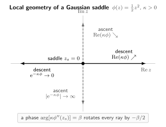
For $\phi(z)=z^2/2$ and positive $\kappa$, the real axis is the descent thimble: $\operatorname{Re}(\kappa\phi)$ increases away from the saddle and $\ee^{-\kappa\phi}$ decays. The dashed imaginary axis is the ascent direction, along which the same exponential grows. If $\arg[\kappa\phi''(z_s)]=\beta$, all four rays rotate by $-\beta/2$.

Leading Stirling from a non-Gaussian integral

The Gaussian lemma becomes useful only after a non-Gaussian exponent has been reduced near its saddle. For real $z>0$, Euler’s integral and the scaling $t=zs$ give

$$\begin{aligned} \Gamma(z) &= \int_0^\infty t^{z-1}\ee^{-t}\,\dd t \\ &= z^z \int_0^\infty \ee^{-z(s-\log s)} \frac{\dd s}{s}. \end{aligned}$$

Here

$$\phi(s)=s-\log s, \qquad a(s)=\frac1s.$$

The positive contour passes through the unique saddle $s=1$, where

$$\phi(1)=1, \qquad \phi''(1)=1, \qquad a(1)=1.$$

The oriented real contour selects the positive Gaussian root, so

$$\Gamma(z) \sim \sqrt{2\pi}\, z^{z-1/2}\ee^{-z}.$$

The original integral is not Gaussian; only its local normal form is. Expanding $\phi$ and $a$ to higher order generates the coefficients $1/(12z),1/(288z^2),\ldots$. For complex $z$, rotating the contour requires the branch and sector data already recorded in the Gamma section.

Which saddles actually contribute?

Local saddle data do not decide the global contour. In relative homology, an admissible contour decomposes schematically as

$$[\Gamma] = \sum_s n_s[\mathcal J_s], \qquad n_s\in\mathbb Z,$$

where $\mathcal J_s$ is a downward thimble and $n_s$ is its intersection number with the dual upward cycle. Endpoints, poles, and branch points are part of the relative problem. A saddle with $n_s=0$ does not contribute even if its exponential is large.

Thimble decompositions can jump when saddles are connected by a constant-phase trajectory. A necessary phase-alignment condition for such a connection is

$$\operatorname{Im} \left[ \kappa\bigl(\phi(z_s)-\phi(z_t)\bigr) \right] =0.$$

It is not sufficient: an actual global connecting flow must exist, and the relevant intersection data must change.

Equality of exponential magnitudes instead tests the real part. Because the names “Stokes line” and “anti-Stokes line” are interchanged in the literature, the book states the relevant real or imaginary condition rather than relying on the name.

Coalescing saddles, a saddle meeting an endpoint, or a saddle meeting a pole invalidate the isolated Gaussian approximation. They require a uniform local model—typically Airy, parabolic-cylinder, or another canonical integral—and a new scaling limit.

The large-order recurrence page applies the same saddle logic to recurrence integrals, while the instanton and large-order page tracks the corresponding exponential scales in transseries.

Borel–Laplace summation in the house convention

Let

$$\widehat f(\hbar) = a_0+\sum_{n\geq1}a_n\hbar^n.$$

Gevrey-1 growth means that some $C,A>0$ obey

$$|a_n|\leq CA^n\Gamma(n+1).$$

The book removes the constant term and uses the shifted Borel transform

$$\mathcal B\widehat f(\xi) := \sum_{n\geq1} \frac{a_n}{\Gamma(n)} \xi^{n-1}.$$

Suppose this germ continues along $\arg\xi=\theta$ and, for large $t>0$, obeys a bound for some $C_B>0$ and $\sigma\geq0$,

$$\left| \mathcal B\widehat f(\ee^{\ii\theta}t) \right| \leq C_B\ee^{\sigma t}.$$

Its directional Laplace transform is

$$\mathcal S_\theta\widehat f(\hbar) := a_0+ \int_0^{\ee^{\ii\theta}\infty} \ee^{-\xi/\hbar} \mathcal B\widehat f(\xi)\,\dd\xi,$$

where

$$\operatorname{Re} \left( \frac{\ee^{\ii\theta}}{\hbar} \right)>\sigma$$

is the corresponding tangent-domain condition. The weaker inequality $>0$ suffices only for exponential type zero. There is no factor $1/\hbar$ in this shifted convention. Indeed,

$$\int_0^{\ee^{\ii\theta}\infty} \ee^{-\xi/\hbar} \frac{\xi^{n-1}}{\Gamma(n)} \,\dd\xi = \hbar^n.$$

Many sources instead use

$$\mathcal B_0\widehat f(\xi) = \sum_{n\geq0} \frac{a_n}{n!}\xi^n$$

and invert with

$$\frac1\hbar \int_0^{\ee^{\ii\theta}\infty} \ee^{-\xi/\hbar} \mathcal B_0\widehat f(\xi)\,\dd\xi.$$

The conversion is

$$\mathcal B\widehat f = \partial_\xi\mathcal B_0\widehat f.$$

Mixing the shifted transform with the unshifted inverse shifts every power by one. Testing the monomial $\hbar^n$ detects the error immediately.

A one-pole lateral jump

The factorial series

$$\widehat F(\hbar) = \sum_{n\geq0}n!\,\hbar^{n+1}$$

has shifted Borel transform

$$\mathcal B\widehat F(\xi) = \frac{1}{1-\xi}.$$

The positive ray meets its pole. Let $\mathcal S_{0+}$ approach the ray from the upper half-plane and $\mathcal S_{0-}$ from the lower half-plane, both oriented from zero to infinity. For $\hbar>0$,

$$\mathcal S_{0+}\widehat F - \mathcal S_{0-}\widehat F = 2\pi\ii\,\ee^{-1/\hbar}.$$

More generally, set $\operatorname{Disc}_\theta=\mathcal S_{\theta+}-\mathcal S_{\theta-}$. If a simple pole at $A$ is the only obstruction between the two lateral contours, the connecting arcs contribute no boundary term, and its Borel residue is $r$, then

$$\operatorname{Disc}_\theta\widehat f = -2\pi\ii\,r\,\ee^{-A/\hbar}.$$

The minus sign comes from the clockwise contour obtained by upper-forward minus lower-forward. In the factorial example $r=-1$, which gives the positive jump above.

This residue calculation exhibits the information invisible to the formal power series: the two sums differ by an exponentially flat term. For a cut or several singularities, the discontinuity is computed from the continued Borel transform, not from a finite Taylor list.

Layer	What has actually been constructed
Formal series	A coefficient sequence
Borel germ	A convergent function near $\xi=0$ after a Gevrey bound
Continued Borel transform	Analytic data along a specified path or lateral ray
Directional sum	A Laplace integral with growth and decay control
Borel–Padé value	A finite numerical approximation, not automatically a certified sum

The rigorous hierarchy is developed on the exact-WKB summability page. The resurgent-singularity page continues from simple poles to logarithmic and branch-point discontinuities, while the Borel–Padé laboratory separates continuation error, quadrature error, and spectral root finding.

Quadratic differentials, covers, and homology

A meromorphic quadratic differential is locally

$$\varphi=Q(z)(\dd z)^2.$$

Under $z=z(w)$ its coefficient transforms as

$$\widetilde Q(w) = Q(z(w)) \left( \frac{\dd z}{\dd w} \right)^2.$$

Its square root becomes a one-form on the normalized spectral cover

$$\widehat\Sigma: \qquad \lambda^2=\varphi.$$

Locally $\lambda=y\,\dd z$ and $y^2=Q(z)$. A zero or pole of $\varphi$ of odd order is a branch point of the normalized double cover. The deck involution $\iota$ reverses the one-form:

$$\iota^*\lambda=-\lambda.$$

Hence the same projected path on the opposite sheet has the opposite action.

On a simply connected chart of $\widehat\Sigma$ away from critical points, choose a sheet and base point $p_0$. The distinguished local coordinate is

$$w(p)=\int_{p_0}^{p}\lambda.$$

In the book’s Schrödinger normalization the leading WKB differential is

$$\varphi_0 = R_0(z)(\dd z)^2, \qquad R_0=V_0-E.$$

For exact-WKB phase $\theta$,

$$\varphi_\theta = \ee^{-2\ii\theta}\varphi, \qquad w_\theta = \ee^{-\ii\theta}w.$$

Horizontal trajectories satisfy

$$\operatorname{Im}w_\theta = \text{constant}.$$

If

$$\varphi = c(z-z_0)^m(\dd z)^2 \left[1+O(z-z_0)\right], \qquad m\geq1,$$

then

$$w-w_0 \sim \frac{2\sqrt c}{m+2} (z-z_0)^{(m+2)/2}.$$

There are $m+2$ horizontal prongs at that zero; a simple turning point has three.

Closed periods and open connection paths

Let $S$ be the lifted poles or other deleted points and set $\widehat X=\widehat\Sigma\setminus S$. Closed cycles lie in

$$H_1(\widehat X,\mathbb Z).$$

With $\Pi_\gamma=\oint_\gamma\lambda$, oddness gives

$$\Pi_{\iota_*\gamma} = -\Pi_\gamma.$$

Invariant cycles therefore have zero period. Over $\mathbb Q$, the period of an arbitrary cycle is determined by its anti-invariant projection

$$\gamma^-_{\mathbb Q} := \frac12 \left( \gamma-\iota_*\gamma \right), \qquad \Pi_\gamma=\Pi_{\gamma^-_{\mathbb Q}}.$$

That projection need not be integral. The natural integral charge lattice is

$$\begin{aligned} \Gamma^- &:= \ker\!\left( 1+\iota_*: H_1(\widehat X,\mathbb Z) \to H_1(\widehat X,\mathbb Z) \right) \\ &= \left\{ \gamma:\iota_*\gamma=-\gamma \right\}. \end{aligned}$$

Paths ending in a marked set $P$ lie in

$$H_1(\widehat X,P;\mathbb Z).$$

The boundary map remembers the signed endpoints:

$$\partial: H_1(\widehat X,P;\mathbb Z) \longrightarrow H_0(P;\mathbb Z).$$

A closed WKB period and an open connection action therefore belong to different groups. Deforming either across a pole of $\lambda$ changes the integral by the appropriate $2\pi\ii$ times residue; compactification does not erase that obstruction.

There is an integral factor-of-two trap. If an open lift $\beta$ has endpoints fixed by $\iota$, its anti-invariant closed lift obeys

$$\int_{\beta-\iota_*\beta}\lambda = 2\int_\beta\lambda.$$

If $\gamma$ is already anti-invariant, applying $1-\iota_*$ produces $2\gamma$, not a new primitive representative.

If a connected degree-two cover of a compact genus-$g$ surface has $r$ simple branch points, Riemann–Hurwitz gives

$$2g(\widehat\Sigma)-2 = 2(2g-2)+r.$$

Thus a four-branch-point cover of the sphere has genus one. An oriented symplectic basis is still extra data: the branch-cut drawing does not decide which representatives are $A$ and $B$ or how they are oriented. The book fixes their order and orientation by $\langle A,B\rangle=+1$.

The spectral-cover page derives the branch and genus rules. The cycle and residue toolkit develops absolute and relative periods, and the Stokes-graph page connects the phased foliation to sectorial WKB solutions.

A compact decision ledger

Task	Data that make it well posed	Fast audit
Continue a local solution	Germ, base point, punctured domain, path	Round trip around one generator
Simplify a Gamma product	Exact identity, excluded poles, logarithm branch	Compare recurrence at a shifted argument
Evaluate a saddle integral	Large-parameter sector, oriented contour, contributing thimbles	Rotated Gaussian benchmark
Borel sum a formal tail	Transform convention, continued germ, ray, lateral side, growth bound	Reconstruct one monomial
Integrate a WKB form	Normalized cover, sheet, cycle or relative path, orientation, residues	Apply the deck involution and one intersection check

Common pitfalls

Treating a branch cut as an intrinsic boundary. Moving a cut changes a planar representative, not the covering surface. Carry the lifted path and sheet label through the move.

Using Stirling’s series across its excluded ray. The negative axis is where the selected logarithm and exponentially improved terms require special care. Use recurrence or reflection first and state the sector of the remaining expansion.

Choosing the Gaussian square root without the contour. The Hessian determines two square roots, while the oriented thimble selects one. Reversing the contour reverses the saddle contribution.

Calling a finite Borel polynomial a Borel sum. A coefficient list gives a local approximation to a germ. Analytic continuation, lateral choice, Laplace growth, and numerical error remain separate questions.

Identifying a projected loop with a cycle on the cover. The sheet, orientation, deleted poles, and endpoint set can change the period even when the planar drawing looks unchanged.

Exercises

1. Continue a two-branch power

At the base point $z_*=1/2$, choose the principal values of

$$f(z)=z^\alpha(1-z)^\beta.$$

Find the multiplier after a positive loop around $0$ that does not enclose $1$, and after a positive loop around $1$ that does not enclose $0$.

Solution

Around the first loop, $\operatorname{Log}z$ gains $2\pi\ii$ while $\operatorname{Log}(1-z)$ returns to its original branch. Therefore

$$f\longmapsto\ee^{2\pi\ii\alpha}f.$$

Around the second loop, $1-z$ winds once positively around zero, so

$$f\longmapsto\ee^{2\pi\ii\beta}f.$$

The multipliers commute because this scalar example has an Abelian one-dimensional monodromy representation. The corresponding matrix problem need not commute.

2. Check an exact Gamma ratio against Stirling

Use recurrence to evaluate

$$\frac{\Gamma(z+3/2)}{\Gamma(z+1/2)}$$

exactly. Then recover its first two large-$z$ terms from the ratio card.

Solution

Recurrence gives

$$\Gamma\left(z+\frac32\right) = \left(z+\frac12\right) \Gamma\left(z+\frac12\right),$$

hence the exact ratio is $z+1/2$. In the asymptotic formula take $a=3/2$ and $b=1/2$. Then

$$a-b=1, \qquad a+b-1=1,$$

so

$$\frac{\Gamma(z+3/2)}{\Gamma(z+1/2)} \sim z\left(1+\frac{1}{2z}+O(z^{-2})\right) = z+\frac12+O(z^{-1}).$$

The apparent remainder vanishes identically because recurrence already gave the exact polynomial.

3. Calibrate a rotated Gaussian contour

For $\kappa>0$, consider

$$I_\alpha(\kappa) = \int_{\ee^{\ii\alpha}\mathbb R} \ee^{-\kappa z^2/2}\,\dd z,$$

with the contour oriented by $z=\ee^{\ii\alpha}x$ as $x:-\infty\to+\infty$. Determine the absolute-convergence sectors and evaluate the integral for $|\alpha|<\pi/4$.

Solution

Along the contour,

$$\left| \ee^{-\kappa z^2/2} \right| = \exp\left[ -\frac{\kappa x^2}{2}\cos(2\alpha) \right].$$

The integral converges absolutely with Gaussian decay when $\cos(2\alpha)>0$, namely in the sectors

$$|\alpha-k\pi|<\frac{\pi}{4}, \qquad k\in\mathbb Z.$$

On the boundary $\cos(2\alpha)=0$, the corresponding Fresnel integrals are conditionally convergent, but those rays are not exponentially decaying thimbles.

For $|\alpha|<\pi/4$, rotate the contour to the real axis without leaving the decay sectors. No singularity is crossed and the connecting arcs vanish, so

$$I_\alpha(\kappa) = \sqrt{\frac{2\pi}{\kappa}}.$$

At $\alpha=\pi$ the same geometric line has the opposite orientation and the answer changes sign. This is why the square-root phase cannot be detached from the oriented contour.

4. Derive a lateral Borel jump

For

$$\widehat F(\hbar) = \sum_{n\geq0}n!\hbar^{n+1},$$

derive its shifted Borel transform and the difference between the upper and lower positive-ray sums for $\hbar>0$.

Solution

The coefficient of $\hbar^{n+1}$ is $n!=\Gamma(n+1)$, so

$$\mathcal B\widehat F(\xi) = \sum_{n\geq0}\xi^n = \frac{1}{1-\xi}.$$

The upper contour minus the lower contour is clockwise around the pole at $\xi=1$. Since

$$\operatorname*{res}_{\xi=1} \frac{\ee^{-\xi/\hbar}}{1-\xi} = -\ee^{-1/\hbar},$$

the residue theorem gives

$$\mathcal S_{0+}\widehat F - \mathcal S_{0-}\widehat F = -2\pi\ii\left(-\ee^{-1/\hbar}\right) = 2\pi\ii\ee^{-1/\hbar}.$$

The jump has zero formal power series at $\hbar=0$ in the positive decay sector.

5. Audit a phased branch-arc lift

Let

$$\varphi = (z^2-1)(\dd z)^2,$$

and choose the sheet on which $\lambda=+\ii\sqrt{1-x^2}\,\dd x$ for $-1<x<1$. Let $\beta$ be the lift of the interval from $-1$ to $1$, and set $\gamma=\beta-\iota_*\beta$. Determine the phase $\theta$ for which the projected interval is horizontal, show that $\gamma$ is an anti-invariant closed cycle, and evaluate $\oint_\gamma\lambda$.

Solution

Along the chosen lift,

$$\ee^{-\ii\theta}\lambda = \ee^{-\ii\theta}\ii \sqrt{1-x^2}\,\dd x.$$

This is real when $\theta=\pi/2\pmod\pi$, so the interval is horizontal for those phases. Its endpoints are branch points and hence are fixed by $\iota$. Therefore

$$\partial\gamma = 0, \qquad \iota_*\gamma=-\gamma.$$

Finally,

$$\begin{aligned} \oint_\gamma\lambda &= 2\int_\beta\lambda \\ &= 2\ii\int_{-1}^{1}\sqrt{1-x^2}\,\dd x \\ &= \ii\pi. \end{aligned}$$

The middle line is the factor-of-two rule, and the last integral is twice the area of a unit semicircle. Reversing the chosen sheet or the cycle orientation reverses the answer.

References

• NIST DLMF, §1.10 Functions of a Complex Variable, §4.2 Logarithm, Exponential, and Powers, §5.2 Gamma Definition and Analytic Properties, §5.5 Gamma Functional Relations, §5.11 Gamma Asymptotics, and §2.4 Contour Integrals, for the branch, Gamma, Stirling, and saddle-point reference formulae.
• F. W. J. Olver, Asymptotics and Special Functions, for uniform asymptotic expansions, contour methods, and error bounds.
• E. Witten, “Analytic Continuation of Chern–Simons Theory”, for downward and upward cycles, intersection coefficients, and Picard–Lefschetz jumps.
• W. Balser, From Divergent Power Series to Analytic Functions, Lecture Notes in Mathematics 1582 (1994), for Borel–Laplace and multisummability theory.
• D. Sauzin, “Introduction to 1-Summability and Resurgence”, for a detailed modern treatment of Borel germs, lateral sums, and singularities.
• K. Strebel, Quadratic Differentials, for natural coordinates and trajectory structures.
• T. Bridgeland and I. Smith, “Quadratic Differentials as Stability Conditions”, for spectral covers, anti-invariant homology, and period coordinates.
• A. Hatcher, Algebraic Topology, Chapter 2, for absolute and relative homology.