The Omega Background and Nekrasov Partition Function

Page 2 constructed an undeformed Seiberg–Witten family: a curve, a meromorphic differential, integral cycles, and period coordinates $(a_D,a)$. The Omega background changes the calculation. It places the four-dimensional theory in a two-parameter equivariant spacetime, makes the instanton integrals well defined after localization, and packages their answers into a meromorphic function of $(\epsilon_1,\epsilon_2)$.

That function is not yet a wavefunction, a quantum curve, or a spectrum. At generic $(\epsilon_1,\epsilon_2)$ it is a protected equivariant partition function. Its instanton part is an infinite sum over fixed points labeled by Young diagrams; its logarithm recovers the classical prepotential only after a simultaneous undeformed limit. Page 4 will take a different, anisotropic limit. Pages 5–6 will then supply the operator and period data needed before one may identify $\epsilon_1$ with a spectral $\hbar$.

Page question

What does the two-parameter Omega deformation compute, how does equivariant localization reduce it to colored partitions, and which limits and convention maps are still required before it can enter a quantum-ODE dictionary?

Status ledger

Statement used on this page	Status
The generic Omega background has two independent equivariant weights	Defining datum
$Q_\Omega^2$ generates rotations, gauge transformations, and flavor transformations	Exact schematic equivariant statement; generator signs depend on convention
Instanton integrals reduce to torus-fixed data	Exact in localized equivariant cohomology after the moduli-space prescription is fixed
Fixed points are labeled by $N$-tuples of Young diagrams	Exact for resolved framed $U(N)$ ADHM moduli at generic weights
$Z_{\mathrm{Nek}}=Z_{\mathrm{cl}}Z_{\mathrm{1-loop}}Z_{\mathrm{inst}}$	Exact definition in the scheme declared below
The three factors are separately scheme-independent	False
The instanton sum includes every nonnegative instanton number	Exact as a formal series in $\mathfrak q$
“All instantons” means a complete nonperturbative ODE spectrum	False
The undeformed limit of $\epsilon_1\epsilon_2\log Z$ gives a localization-normalized prepotential	Exact coefficientwise; in this page’s package it equals $-2\pi\ii\mathcal F_{\mathrm{SW}}$ after scale and counterterm matching
The self-dual slice $\epsilon_1+\epsilon_2=0$ is the NS limit	False
The NS limit is obtained by substituting $\epsilon_2=0$ into $Z$	False; $Z$ is generally exponentially singular there
$\epsilon_1=\hbar$	Model-dependent identification deferred to Pages 5–6
The bulk partition function alone supplies a quantum-curve wavefunction	False in general; a defect or another observable may be required

One name hides three different calculations

We reserve the name full Nekrasov partition function for

$$Z_{\mathrm{Nek}} = Z_{\mathrm{cl}} Z_{\mathrm{1-loop}} Z_{\mathrm{inst}}.$$

The factors have different origins:

Factor	What it records	Normalization issue
$Z_{\mathrm{cl}}$	The classical gauge action evaluated at the Coulomb boundary value	Depends on the trace, coupling, and overall prepotential convention
$Z_{\mathrm{1-loop}}$	The regularized equivariant determinant of perturbative fluctuations	Depends on the regulator and local counterterms
$Z_{\mathrm{inst}}$	Positive-instanton sectors localized on resolved moduli spaces	Depends on the instanton fugacity, mass labels, compactification, and any decoupled Abelian factor

Many papers use $Z_{\mathrm{Nek}}$ for the third factor alone. That abbreviation is harmless only when it is announced. Here

$$Z_{\mathrm{inst}}(\mathfrak q=0)=1,$$

and an expression called $Z_{\mathrm{Nek}}$ always includes all three factors unless a superscript such as “inst” is shown.

The variables also belong to different layers:

$$Z_{\mathrm{Nek}} = Z_{\mathrm{Nek}} \left( \boldsymbol a, \boldsymbol\mu, \mathfrak q; \epsilon_1,\epsilon_2 \right).$$

$\boldsymbol a$ chooses a Coulomb vacuum in a local electric frame, $\boldsymbol\mu$ denotes the equivariant mass labels used in the localization formula, and $\mathfrak q$ counts instanton number. The two $\epsilon$‘s deform spacetime. None is an ODE energy.

Convention ledger

Datum	Convention on this page
Spacetime	Euclidean $\mathbb C^2$ with coordinates $(z_1,z_2)$
Rotation weights	$(z_1,z_2)\mapsto(e^{t\epsilon_1}z_1,e^{t\epsilon_2}z_2)$
Sum of weights	$\epsilon_\Sigma:=\epsilon_1+\epsilon_2$; no ambiguous symbol $\epsilon_+$
Dimensions	$[a_\alpha]=[\mu_f]=[\epsilon_i]=1$
Gauge combinatorics	Framed $U(N)$ ADHM data, followed by $\sum_\alpha a_\alpha=0$ on the interacting $SU(N)$ slice
Pure-$SU(2)$ frame	$(a_1,a_2)=(a,-a)$, so a root has mass parameter $2a$
Instanton fugacity	$\mathfrak q=q_{\mathrm{UV}}$ if $b_0=0$; $\mathfrak q=\Lambda_{\mathrm{Nek}}^{b_0}$ if $b_0>0$
Diagram coordinates	$s=(i,j)$ means row $i$, column $j$
Fixed-point normalization	The empty tuple contributes one
Full function	$Z_{\mathrm{Nek}}:=Z_{\mathrm{cl}}Z_{\mathrm{1-loop}}Z_{\mathrm{inst}}$
Localization free energy	$\mathscr F_\Omega:=\epsilon_1\epsilon_2\log Z_{\mathrm{Nek}}$
Period normalization	$\mathscr F_0=-2\pi\ii\,\mathcal F_{\mathrm{SW}}$ in the fixed-point/Barnes package used here
NS operation	First form $\log Z$; then take $\epsilon_2\to0$ with $\epsilon_1$ fixed—Page 4

The scale $\Lambda_{\mathrm{Nek}}$ is initially a localization-scheme scale. Its relation to the curve-normalized $\Lambda$ of Page 2 can contain a finite constant or phase. In the pure-$SU(2)$ calculation below, a two-instanton comparison calibrates the two conventions and sets $\mathfrak q=\Lambda^4$.

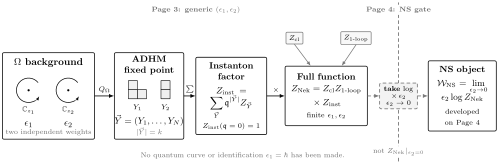
At generic $(\epsilon_1,\epsilon_2)$, equivariant localization replaces each instanton-moduli integral by a sum over Young-diagram fixed points. Those weights build only $Z_{\mathrm{inst}}$; the classical and one-loop factors complete $Z_{\mathrm{Nek}}$. The dashed Page 4 gate emphasizes that $\mathcal W_{\mathrm{NS}}$ comes from $\epsilon_2\log Z_{\mathrm{Nek}}$, not from setting $\epsilon_2=0$ inside $Z_{\mathrm{Nek}}$.

The Ω background rotates two complex planes

Write

$$\mathbb R^4 \simeq \mathbb C_{z_1}\times\mathbb C_{z_2}.$$

The complexified spacetime torus acts by

$$(z_1,z_2) \longmapsto \left( \ee^{t\epsilon_1}z_1, \ee^{t\epsilon_2}z_2 \right).$$

For literal compact rotations one takes an appropriate real slice and writes phases. The final holomorphic formulas are meromorphic in complex $\epsilon_i$ and are continued away from that slice. Both parameters have mass dimension one because they multiply angular momenta in an exponent with an inverse-length parameter.

A concrete construction starts in five dimensions. Form a mapping torus by identifying

$$\begin{aligned} (z_1,z_2,x^5) \sim \bigl( &\ee^{\ii\beta\epsilon_1}z_1, \ee^{\ii\beta\epsilon_2}z_2, \\ &x^5+\beta \bigr). \end{aligned}$$

Gauge and flavor holonomies around the circle insert $\ee^{\ii\beta a}$ and $\ee^{\ii\beta\mu}$. Preserving the desired supercharge also requires an $SU(2)_R$ twist; in a standard convention its eigenvalues are

$$\ee^{\pm\ii\beta\epsilon_\Sigma/2}.$$

The supersymmetric trace is schematically

$$\begin{aligned} Z(\beta) = \operatorname{Tr}_{\mathcal H} (-1)^F \exp\!\Bigg[ \ii\beta\Bigg( &\epsilon_1J_1+ \epsilon_2J_2 \\ &+ \sum_\alpha a_\alpha Q_\alpha + \sum_f\mu_fF_f \Bigg) \Bigg]. \end{aligned}$$

In this trace, $J_1$ and $J_2$ denote the rotation generators after the required Lorentz–$R$ twist has been combined with them. Writing untwisted angular momenta instead would require displaying the $R$-charge insertion separately.

The four-dimensional cohomological partition function arises from the $\beta\to0$ limit with the additive weights held fixed. For an asymptotically free theory, one must simultaneously scale the classical five-dimensional instanton weight. In the convention of the mapping- torus derivation,

$$\exp\!\left( -\frac{8\pi^2\beta}{g_{5\mathrm d}^2} \right) = (-\ii\beta)^{b_0} \mathfrak q,$$

with $\mathfrak q$ fixed; a phase can instead be absorbed into the definition of $\mathfrak q$. For $SU(N)$ with $N_f$ fundamental full hypermultiplets, $b_0=2N-N_f$. A genuinely five-dimensional, K-theoretic partition function instead retains multiplicative factors such as $1-\ee^{-\beta w}$. These are related limits, not interchangeable formulas.

Four regimes must remain separate:

Regime	Operation	Object emphasized
Generic Omega background	$\epsilon_1,\epsilon_2$ independent	Two-parameter equivariant partition function
Undeformed or flat limit	$\epsilon_1,\epsilon_2\to0$ together	Seiberg–Witten prepotential
Self-dual or unrefined slice	$\epsilon_\Sigma=0$	A one-parameter specialization of $Z$
Nekrasov–Shatashvili limit	$\epsilon_2\to0$ with $\epsilon_1$ fixed	Twisted superpotential after taking $\log Z$

The self-dual slice approaches the origin along $(\epsilon_1,\epsilon_2)=(\hbar,-\hbar)$ if $\hbar\to0$. The NS limit instead approaches the $\epsilon_1$ axis at nonzero $\epsilon_1$. They coincide only at the undeformed endpoint.

Equivariant supersymmetry replaces volume by fixed points

The preserved supercharge is not ordinarily nilpotent on every field. Rather, in a conventional cohomological presentation,

$$Q_\Omega^2 = \mathcal L_V + \delta_{\mathrm{gauge}}(\boldsymbol a) + \delta_{\mathrm{flavor}}(\boldsymbol\mu),$$

up to convention-dependent signs and an $R$-symmetry term already absorbed into the background. Here $V$ generates the two rotations. On observables invariant under the combined action, the right-hand side vanishes. That equivariant nilpotence is enough for the standard localization argument: a $Q_\Omega$-exact deformation changes neither the protected integral nor its fixed-point answer.

Even the equivariant volume of spacetime illustrates the mechanism. With the orientation convention used here,

$$\int_{\mathbb C^2}^{T^2}1 = \frac{1}{\epsilon_1\epsilon_2}.$$

The ordinary volume is infinite. Its equivariant pushforward is the reciprocal Euler class of the tangent representation at the unique spacetime fixed point $z_1=z_2=0$. This effective volume explains why the logarithm of a four-dimensional local partition function begins as

$$\log Z \sim \frac{\text{local effective density}} {\epsilon_1\epsilon_2}.$$

For any smooth $T$-space with isolated fixed points, the corresponding localization formula is

$$\int_M^T\alpha = \sum_{p\in M^T} \frac{\alpha|_p} {e_T(T_pM)}.$$

This equality is taken in localized equivariant cohomology, where the tangent weights have been inverted. For a noncompact moduli space it defines an equivariant pushforward; it is not a claim that the ordinary integral of $1$ converges.

For instanton number $k$, let $\widetilde{\mathcal M}_{N,k}$ denote the chosen resolved moduli space of framed $U(N)$ instantons. The schematic instanton expansion is

$$\begin{aligned} Z_{\mathrm{inst}} &= \sum_{k\geq0} \mathfrak q^k \int_{\widetilde{\mathcal M}_{N,k}}^T e_T(\mathcal E_{\mathrm{matter}}) \\ &= \sum_{k\geq0} \mathfrak q^k \sum_{p\in\widetilde{\mathcal M}_{N,k}^T} \frac{ e_T(\mathcal E_{\mathrm{matter}}|_p) }{ e_T(T_p\widetilde{\mathcal M}_{N,k}) }. \end{aligned}$$

The vector multiplet supplies the reciprocal tangent Euler class. Matter supplies numerator Euler classes of index bundles. More general quivers can also be written as contour integrals; then the contour or Jeffrey–Kirwan chamber is part of the definition.

ADHM resolution makes the fixed points discrete

The ordinary instanton moduli space has small-instanton singularities, so applying the smooth fixed-point formula to it without qualification would be wrong. For framed $U(N)$ instantons, introduce complex vector spaces

$$V\simeq\mathbb C^k, \qquad W\simeq\mathbb C^N,$$

and ADHM data

$$\begin{gathered} B_1,B_2\in\operatorname{End}(V), \\ I\in\operatorname{Hom}(W,V), \qquad J\in\operatorname{Hom}(V,W). \end{gathered}$$

They obey the complex moment-map equation

$$[B_1,B_2]+IJ=0$$

together with a stability condition, and are quotiented by $GL(V)$. Equivalently, a nonzero real Fayet–Iliopoulos or noncommutativity parameter resolves the small-instanton locus. The complex dimension follows before any detailed geometry is used:

$$\begin{aligned} \dim_{\mathbb C} \widetilde{\mathcal M}_{N,k} &= \left(2k^2+2Nk\right) -k^2-k^2 \\ &=2Nk. \end{aligned}$$

The first subtraction imposes the complex equation; the second takes the complex gauge quotient. Stability makes this quotient the resolved space needed by localization.

At generic equivariant parameters, the fixed points of

$$T = T_\Omega^2 \times T_a^N \times T_{\mathrm f}$$

are isolated and labeled by an $N$-tuple of Young diagrams,

$$\boldsymbol Y = (Y_1,\ldots,Y_N), \qquad |\boldsymbol Y| := \sum_{\alpha=1}^N|Y_\alpha| =k.$$

Each color $\alpha$ associates a partition to the Coulomb weight $a_\alpha$. The empty $N$-tuple is the unique $k=0$ fixed point.

For $U(1)$, the algebraic reason partitions appear is especially concrete. A torus-invariant ideal in $\mathbb C[z_1,z_2]$ is generated by monomials. The monomials not contained in the ideal form a finite downward-closed set in the exponent lattice, hence a Ferrers diagram. Framing by the $N$ Coulomb weights colors this construction and produces the $N$-tuple $\boldsymbol Y$.

Three unrelated uses of “fixed point”

The origin of $\mathbb C^2$ is fixed by the spacetime rotations. A colored partition labels a fixed point of the induced torus action on an instanton moduli space. A zero of the Page 2 discriminant is instead a singular vacuum on the Coulomb branch. These three statements live in different spaces and must not be identified.

Colored partitions encode the tangent Euler class

It is useful to see once how the geometry becomes combinatorics. Let $e^w$ denote the formal character of a one-dimensional representation of additive weight $w$. At the fixed point $\boldsymbol Y$, one convention gives

$$W = \sum_{\alpha=1}^N \ee^{a_\alpha},$$

and

$$V_{\boldsymbol Y} = \sum_{\alpha=1}^N \sum_{(i,j)\in Y_\alpha} \ee^{ a_\alpha+(i-1)\epsilon_1+(j-1)\epsilon_2 }.$$

The tangent character can then be written compactly as

$$\begin{aligned} T_{\boldsymbol Y} \widetilde{\mathcal M}_{N,k} = {}&V_{\boldsymbol Y}^*W + \ee^{\epsilon_\Sigma} W^*V_{\boldsymbol Y} \\ &- (1-\ee^{\epsilon_1}) (1-\ee^{\epsilon_2}) V_{\boldsymbol Y}V_{\boldsymbol Y}^*. \end{aligned}$$

Expanding this virtual character into monomials $\sum_r n_r\ee^{w_r}$ turns its Euler class into $\prod_rw_r^{n_r}$. Arm and leg lengths are the factored form of that product.

Write a Young diagram as row lengths $Y=(Y_1\geq Y_2\geq\cdots)$. For a box $s=(i,j)$, define

$$A_Y(s)=Y_i-j, \qquad L_Y(s)=Y_j^T-i.$$

$A_Y(s)$ counts boxes to the right when $s\in Y$, and $L_Y(s)$ counts boxes below. In a mixed expression such as $L_W(s)$, the box $s$ need not lie in $W$; the generalized leg length may therefore be negative. Replacing it by zero is a common implementation bug.

Define

$$E(x;Y,W;s) := x - \epsilon_1L_W(s) + \epsilon_2\bigl(A_Y(s)+1\bigr),$$

and the two-diagram Nekrasov factor

$$\begin{aligned} N_{Y,W}(x) :={}& \prod_{s\in Y} E(x;Y,W;s) \\ &\times \prod_{t\in W} \left[ \epsilon_\Sigma -E(-x;W,Y;t) \right]. \end{aligned}$$

The pure-vector fixed-point weight is

$$z_{\mathrm{vec}} (\boldsymbol a,\boldsymbol Y) = \prod_{\alpha,\beta=1}^N \frac{1}{ N_{Y_\alpha,Y_\beta} (a_\alpha-a_\beta) }.$$

Consequently,

$$Z_{\mathrm{inst}}^{\mathrm{pure}\ U(N)} = \sum_{\boldsymbol Y} \mathfrak q^{|\boldsymbol Y|} z_{\mathrm{vec}} (\boldsymbol a,\boldsymbol Y).$$

The formula is first interpreted for generic parameters, where no tangent weight vanishes, and then meromorphically continued. A pole at a resonance such as $a_\alpha-a_\beta=r\epsilon_1+s\epsilon_2$ is a degenerating equivariant weight. It is not automatically a physical Seiberg–Witten discriminant point.

Omega-plane exchange is visible only after transposing every diagram:

$$(\epsilon_1,\epsilon_2,Y_\alpha) \longleftrightarrow (\epsilon_2,\epsilon_1,Y_\alpha^T).$$

This is a valuable check on a symbolic implementation.

Matter factors require a mass ledger

For a box $s=(i,j)$, set

$$\phi(a,s) = a+ \epsilon_1(i-1)+ \epsilon_2(j-1).$$

In the convention used by the fixed-point formulas on this page, a fundamental and an antifundamental label contribute

$$z_{\mathrm{fund}} (\boldsymbol a,\boldsymbol Y;\mu) = \prod_{\alpha=1}^N \prod_{s\in Y_\alpha} \left[ \phi(a_\alpha,s)-\mu+\epsilon_\Sigma \right],$$

and

$$\begin{aligned} z_{\mathrm{antifund}} (\boldsymbol a,\boldsymbol Y;\mu) &= z_{\mathrm{fund}} (\boldsymbol a,\boldsymbol Y;\epsilon_\Sigma-\mu) \\ &= \prod_{\alpha=1}^N \prod_{s\in Y_\alpha} \left[ \phi(a_\alpha,s)+\mu \right]. \end{aligned}$$

For two gauge nodes, a bifundamental of equivariant mass $\mu$ has

$$\begin{aligned} z_{\mathrm{bifund}} ={}& \prod_{\alpha,\beta} \prod_{s\in Y_\alpha} \left[ E(a_\alpha-b_\beta;Y_\alpha,W_\beta;s)-\mu \right] \\ &\times \prod_{\alpha,\beta} \prod_{t\in W_\beta} \Bigl[ \epsilon_\Sigma -E(b_\beta-a_\alpha;W_\beta,Y_\alpha;t) -\mu \Bigr]. \end{aligned}$$

An adjoint is the specialization $(\boldsymbol b,\boldsymbol W)=(\boldsymbol a,\boldsymbol Y)$, and

$$z_{\mathrm{vec}} = \frac{1}{z_{\mathrm{adj}}(\mu=0)}.$$

These relations are safer than memorizing unrelated matter formulas. They also expose the convention issue. A commonly used centered mass is

$$\widehat m = \mu- \frac{\epsilon_\Sigma}{2}.$$

Other authors call either $\mu$, $\widehat m$, or its negative the physical mass. The Page 1 central-charge mass is not to be inserted into a printed fixed-point formula until this translation has been checked. The shift vanishes in the simultaneous undeformed limit but is essential at finite deformation and in AGT.

With matter present, the complete instanton factor takes the form

$$Z_{\mathrm{inst}} = \sum_{\boldsymbol Y} \mathfrak q^{|\boldsymbol Y|} z_{\mathrm{vec}} \prod_f z_{\mathrm{matter},f},$$

with one such factor per hypermultiplet or quiver edge.

Pure SU(2) at one instanton

Localization naturally computes the resolved framed $U(2)$ problem. Write

$$a_1=a_0+a, \qquad a_2=a_0-a, \qquad \Delta:=a_1-a_2=2a.$$

Every pure-vector factor depends only on differences, so the diagonal coordinate $a_0$ drops out. The two one-instanton fixed points are

$$(\Box,\varnothing), \qquad (\varnothing,\Box).$$

The elementary factors are

$$\begin{gathered} N_{\Box,\Box}(0) = \epsilon_1\epsilon_2, \\ N_{\Box,\varnothing}(x) =x+\epsilon_\Sigma, \qquad N_{\varnothing,\Box}(x) =x. \end{gathered}$$

Therefore the two colored boxes contribute

$$z_{(\Box,\varnothing)} = -\frac{1}{ \epsilon_1\epsilon_2 \Delta(\Delta+\epsilon_\Sigma) },$$

and

$$z_{(\varnothing,\Box)} = -\frac{1}{ \epsilon_1\epsilon_2 \Delta(\Delta-\epsilon_\Sigma) }.$$

Adding before simplifying gives

$$\begin{aligned} Z_{\mathrm{inst}}^{\mathrm{pure}\ SU(2)} = 1 - \mathfrak q\, \frac{2}{ \epsilon_1\epsilon_2 \left[ 4a^2-(\epsilon_1+\epsilon_2)^2 \right] } +O(\mathfrak q^2). \end{aligned}$$

Three checks are immediate:

1. it is invariant under the Weyl reflection $a\mapsto-a$;
2. it is invariant under $\epsilon_1\leftrightarrow\epsilon_2$; and
3. for pure $SU(2)$, $[\mathfrak q]=4$, while the displayed coefficient has dimension $-4$.

The sign can look different in a source that sends $\mathfrak q\mapsto-\mathfrak q$, reverses an Euler-class orientation, or uses $4a^2-\epsilon_\Sigma^2$ rather than $\epsilon_\Sigma^2-4a^2$ as the displayed denominator. Only a complete convention package can be compared.

Two-instanton checksum

Write

$$Z_{\mathrm{inst}} = 1+\mathfrak q Z_1+\mathfrak q^2Z_2+O(\mathfrak q^3).$$

The five fixed points at $k=2$ are

$$\begin{gathered} ([2],\varnothing), \quad ([1,1],\varnothing), \quad (\varnothing,[2]), \\ (\varnothing,[1,1]), \quad (\Box,\Box). \end{gathered}$$

Their sum simplifies to

$$\begin{aligned} Z_2 ={}& \frac{ 2\Delta^2 -8\epsilon_1^2 -17\epsilon_1\epsilon_2 -8\epsilon_2^2 }{ \epsilon_1^2\epsilon_2^2 (\Delta^2-\epsilon_\Sigma^2) } \\ &\times \frac{1}{ \left[ \Delta^2-(2\epsilon_1+\epsilon_2)^2 \right] } \\ &\times \frac{1}{ \left[ \Delta^2-(\epsilon_1+2\epsilon_2)^2 \right] }. \end{aligned}$$

Individual same-color terms contain apparent poles at $\epsilon_1=\epsilon_2$; they cancel in the five-term sum. This exact coefficient is a stringent test of arm–leg orientation, generalized negative legs, diagram transposition, and color ordering.

The reduction from $U(2)$ differences to the traceless $SU(2)$ variable is clean in the pure-vector sector. It must not be generalized blindly. With matter or quiver nodes, a decoupled $U(1)$ factor can depend on masses and couplings and can be essential in an AGT comparison.

Classical and one-loop factors complete the local block

For a conformal $U(N)$ theory, use the Page 1 definition

$$q_{\mathrm{UV}} = \ee^{2\pi\ii\tau_{\mathrm{UV}}}.$$

In the fixed-point/Barnes sign package adopted here, and with $(\boldsymbol a,\boldsymbol a)=\sum_\alpha a_\alpha^2$, take

$$Z_{\mathrm{cl}} = \exp\!\left[ - \frac{ \log q_{\mathrm{UV}} }{ 2\epsilon_1\epsilon_2 } (\boldsymbol a,\boldsymbol a) \right].$$

On the pure-$SU(2)$ slice this would read $Z_{\mathrm{cl}}=q_{\mathrm{UV}}^{-a^2/(\epsilon_1\epsilon_2)}$. Indeed,

$$\epsilon_1\epsilon_2 \log Z_{\mathrm{cl}} = -\pi\ii\tau_{\mathrm{UV}} (\boldsymbol a,\boldsymbol a),$$

so the relation $\mathscr F_0=-2\pi\ii\mathcal F_{\mathrm{SW}}$ gives $\mathcal F_{\mathrm{SW,cl}} =\tfrac12\tau_{\mathrm{UV}}(\boldsymbol a,\boldsymbol a)$. On the $SU(2)$ slice this is $\tau_{\mathrm{UV}}a^2$, whose derivative is $2\tau_{\mathrm{UV}}a$. Thus the classical exponent and Page 2 period convention pass an independent normalization check.

In an asymptotically free theory, the cutoff-dependent bare factor and the running one-loop determinant are usually combined into a perturbative factor expressed in terms of $\Lambda_{\mathrm{Nek}}^{b_0}$. One should not insert a dimensionless $q_{\mathrm{UV}}$ where the dimensionful fugacity $\mathfrak q$ is required.

For completeness, one explicit one-loop scheme can be defined with the Barnes double zeta function. For $\operatorname{Re}\nu>2$ in an initial convergence chamber, set

$$\zeta_2 (\nu,x\mid\epsilon_1,\epsilon_2;M) := \sum_{r,s\geq0} \left( \frac{x+r\epsilon_1+s\epsilon_2}{M} \right)^{-\nu},$$

continue meromorphically to $\nu=0$, and define

$$\begin{aligned} \log\Gamma_2 (x\mid\epsilon_1,\epsilon_2;M) := \left. \frac{\partial}{\partial\nu} \zeta_2 (\nu,x\mid\epsilon_1,\epsilon_2;M) \right|_{\nu=0}. \end{aligned}$$

Let

$$\gamma_{\epsilon_1,\epsilon_2}(x) := \log\Gamma_2 (x+\epsilon_\Sigma \mid\epsilon_1,\epsilon_2;M).$$

One standard $U(N)$ library of factors is

$$\begin{aligned} Z_{\mathrm{1-loop}}^{\mathrm{vec}} = \prod_{\alpha<\beta} \exp\!\Bigl[ &-\gamma(a_\alpha-a_\beta-\epsilon_1) \\ &-\gamma(a_\alpha-a_\beta-\epsilon_2) \Bigr], \end{aligned}$$ $$Z_{\mathrm{1-loop}}^{\mathrm{fund}}(\mu) = \prod_\alpha \exp\!\left[ \gamma(a_\alpha-\mu) \right],$$

and

$$\begin{aligned} Z_{\mathrm{1-loop}}^{\mathrm{antifund}}(\mu) = \prod_\alpha \exp\!\left[ \gamma(-a_\alpha+\mu-\epsilon_\Sigma) \right]. \end{aligned}$$

Here every $\gamma$ has the same parameters $(\epsilon_1,\epsilon_2;M)$. These formulas are a declared library, not universal typography: shifting the argument in the definition of $\Gamma_2$, using the inverse Barnes function, or renaming a fundamental as an antifundamental changes the printed expressions. The negative classical exponent and this Barnes library form one coherent package. Replacing only one of them splices two analytic- continuation conventions and reverses the flat-limit comparison.

Changing the Barnes scale or subtraction can multiply $Z$ by the exponential of a polynomial of degree at most two in Coulomb and mass parameters. That is the freedom to add a local counterterm or make a finite coupling redefinition. It does not alter the fixed positive-instanton Euler classes, but it can alter an absolute partition function and later accessory-parameter relations.

The $\mathbb C^2$ function is a local holomorphic block with $\boldsymbol a$ held fixed at infinity. It is not the full path integral on $S^4$, where one glues local contributions and integrates over $\boldsymbol a$ with a contour and measure.

The simultaneous undeformed limit returns special geometry

Define the localization-normalized free energy

$$\mathscr F_\Omega (\boldsymbol a,\boldsymbol\mu,\mathfrak q; \epsilon_1,\epsilon_2) := \epsilon_1\epsilon_2 \log Z_{\mathrm{Nek}}.$$

The relevant flat limit is simultaneous:

$$\epsilon_1=t b_1, \qquad \epsilon_2=t b_2, \qquad t\longrightarrow0,$$

at a fixed generic nonzero ratio $b_1/b_2$. As a formal instanton series and after the perturbative subtraction scheme is fixed,

$$\mathscr F_0 := \lim_{t\to0} \mathscr F_\Omega$$

exists coefficientwise. In the fixed-point/Barnes convention used here, its relation to the Page 2 period-normalized prepotential is

$$\mathscr F_0 = - 2\pi\ii\, \mathcal F_{\mathrm{SW}}, \qquad a_{D,i} = - \frac{1}{2\pi\ii} \frac{\partial\mathscr F_0} {\partial a^i}.$$

The factor $2\pi\ii$ and the overall sign belong to the convention, not to the localization theorem. The minus sign is forced once this page’s Euler classes, negative classical exponent, Barnes determinant, and the Page 2 orientation of $a_D$ are held fixed. Some papers absorb the factor into their symbol for the prepotential or use the opposite sign package. The classical exponent, instanton fugacity, period differential, and weak asymptotics must be translated together.

The logarithm is essential. If

$$Z_{\mathrm{inst}} = 1+\mathfrak qZ_1+\mathfrak q^2Z_2+O(\mathfrak q^3),$$

then

$$\log Z_{\mathrm{inst}} = \mathfrak qZ_1 + \mathfrak q^2 \left( Z_2-\frac12Z_1^2 \right) +O(\mathfrak q^3).$$

At two instantons, the leading $(\epsilon_1\epsilon_2)^{-2}$ pieces of $Z_2$ and $Z_1^2/2$ cancel. The connected free energy retains the single effective-volume pole needed for a finite $\mathscr F_0$.

For the pure-$SU(2)$ fixed-point convention above, the first two instanton terms are

$$\mathscr F_{0,\mathrm{inst}}^{\mathrm{loc}} = -\frac{\mathfrak q}{2a^2} -\frac{5\mathfrak q^2}{64a^6} +O(\mathfrak q^3).$$

Equivalently, the Page 2 prepotential has

$$2\pi\ii\, \mathcal F_{\mathrm{SW,inst}} = \frac{\mathfrak q}{2a^2} +\frac{5\mathfrak q^2}{64a^6} +O(\mathfrak q^3).$$

Page 2 found

$$\begin{aligned} a(u) = \sqrt u \left[ 1 -\frac{\Lambda^4}{4u^2} -\frac{15\Lambda^8}{64u^4} +O\!\left( \frac{\Lambda^{12}}{u^6} \right) \right]. \end{aligned}$$

Inverting gives

$$u(a) = a^2 +\frac{\Lambda^4}{2a^2} +\frac{5\Lambda^8}{32a^6} +O(\Lambda^{12}).$$

The two expansions agree through two instantons after calibrating

$$\mathfrak q=\Lambda^4$$

and using the Matone-type check

$$\begin{aligned} u(a) &= a^2 - \mathfrak q \frac{\partial\mathscr F_{0,\mathrm{inst}}^{\mathrm{loc}}} {\partial\mathfrak q} \\ &= a^2 + \mathfrak q \frac{\partial \left( 2\pi\ii\mathcal F_{\mathrm{SW,inst}} \right) }{\partial\mathfrak q}. \end{aligned}$$

Page 7 will derive and normalize such relations. Here it is used only as an independent calibration of the curve scale and the localization sign.

Recovering the prepotential is still not the same as constructing a quantum curve. The prepotential determines undeformed special-geometry derivatives. A differential operator additionally needs a polarization, ordering, wavefunction or defect observable, parameter map, and boundary conditions.

Why printed formulas differ

Before importing a formula, translate this complete set of choices:

Printed difference	What must be checked
$U(N)$ versus $SU(N)$	Traceless Coulomb slice, trace normalization, and any decoupled $U(1)$ factor
$q$, $-q$, or a finite reparametrization of $q$	Euler-class orientation, ultraviolet scheme, and curve-scale matching
$q_{\mathrm{UV}}$ versus $\Lambda^{b_0}$	Dimensionless conformal coupling versus dimensionful asymptotically free fugacity
$\epsilon_2\mapsto-\epsilon_2$	Rotation convention and whether diagrams or arms and legs must be transposed
$\epsilon_+$	Whether it means $\epsilon_1+\epsilon_2$ or half that sum; this page uses $\epsilon_\Sigma$
$m$, $\mu$, or $m\pm\epsilon_\Sigma/2$	Equivariant, centered, AGT, and central-charge mass conventions
Barnes $\Gamma_2$ versus its inverse	Definition of the regularized determinant and local polynomial subtraction
$Z_{\mathrm{Nek}}$ versus $Z_{\mathrm{inst}}$	Whether classical and one-loop factors have been omitted
$\mathscr F$ versus $\mathcal F_{\mathrm{SW}}$	Overall $2\pi\ii$ and sign convention in the period normalization
Additive weights versus $1-\ee^{-\beta w}$	Four-dimensional cohomological versus five-dimensional K-theoretic partition function

An equality that survives only after changing one line of this table is not a contradiction. An equality asserted without the table is not yet normalization-complete.

The NS limit belongs to the next page

Page 3 keeps $\epsilon_1$ and $\epsilon_2$ finite and independent. The next operation is not $Z_{\mathrm{Nek}}|_{\epsilon_2=0}$. The expected asymptotic form is

$$\log Z_{\mathrm{Nek}} = \frac{ \mathcal W_{\mathrm{NS}} (\boldsymbol a,\boldsymbol\mu;\epsilon_1,\mathfrak q) }{\epsilon_2} +O(1),$$

after any required subtractions. Thus Page 4 will define and analyze

$$\mathcal W_{\mathrm{NS}} = \lim_{\epsilon_2\to0} \epsilon_2 \log Z_{\mathrm{Nek}}$$

with $\epsilon_1$ fixed. If only the instanton factor is used, the result must be called $\mathcal W_{\mathrm{NS}}^{\mathrm{inst}}$.

One must take this limit after summing and taking the logarithm; finite Young diagrams do not individually describe the limiting saddle. The identification $\epsilon_1=\hbar$, the quantum periods, Bethe-vacuum equations, and nonperturbative spectral completion remain deferred.

Common pitfalls

Substituting $\epsilon_2=0$ into a fixed-point formula. Individual weights then develop zeros, while the complete partition function has an exponential $1/\epsilon_2$ asymptotic. The NS object is extracted from $\epsilon_2\log Z$ after summation and regularization.

Calling the self-dual slice the NS limit. The conditions $\epsilon_1+\epsilon_2=0$ and $\epsilon_2\to0$ with $\epsilon_1$ fixed are different paths in parameter space. Results specialized to one cannot be transferred to the other without a new limit.

Forgetting the first two factors of the full function. The instanton series is often the only difficult combinatorial piece, but $Z_{\mathrm{cl}}$ and $Z_{\mathrm{1-loop}}$ contribute to the full prepotential and to later accessory derivatives.

Treating Young diagrams as BPS charges. A colored partition labels a localization fixed point in $\widetilde{\mathcal M}_{N,k}$. It is not an element of the electromagnetic charge lattice of Pages 1–2.

Clipping generalized leg lengths at zero. In $L_W(s)=W_j^T-i$, the comparison box need not belong to $W$. Negative legs are required for the cross-color tangent weights and for the correct one-instanton denominator.

Using a $U(N)$ formula as an $SU(N)$ formula without an audit. The traceless condition is enough for the Coulomb-dependent pure-vector series, but matter and quiver theories can retain nontrivial decoupled Abelian prefactors.

Identifying every equivariant pole with a physical singularity. A zero tangent weight can create a pole at a resonance in $a/\epsilon_i$. A Coulomb-branch singularity is instead determined by the Seiberg–Witten discriminant after the undeformed dictionary is fixed.

Calling a formal all-instanton series a complete spectrum. The sum over all $k$ is nonperturbative in the four-dimensional gauge coupling, but it does not supply ODE boundary data, a resummation prescription, or exponentially small effects in a later spectral $\hbar$.

Exercises

1. Separate the four deformations and limits

Classify the generic Omega background, simultaneous undeformed limit, self-dual slice, and NS limit as subsets or limiting paths in the $(\epsilon_1,\epsilon_2)$ plane. Which implications hold?

Solution

The generic background is a point away from special loci with two independent weights. The undeformed limit approaches $(0,0)$ with both weights tending to zero. The self-dual slice is the line $\epsilon_2=-\epsilon_1$. The NS limit approaches the line $\epsilon_2=0$ while holding a generally nonzero $\epsilon_1$ fixed.

Neither special line implies the other. They intersect only at the origin, and the limiting asymptotics along them differ. A self-dual calculation can subsequently take $\epsilon_1\to0$ and reach the undeformed point; an NS calculation can also take its remaining $\epsilon_1\to0$, but those are two-step limits, not identities of the intermediate objects.

2. Use equivariant nilpotence

Suppose

$$Q_\Omega^2 = \mathcal L_V+ \delta_{\mathrm{gauge}}(a)+ \delta_{\mathrm{flavor}}(\mu).$$

Why can $Q_\Omega$ define a cohomology on protected observables even though it does not square to zero on every field?

Solution

Restrict to observables invariant under the combined spacetime, gauge, and flavor action. On that subspace the right-hand side annihilates an observable $\mathcal O$, so $Q_\Omega^2\mathcal O=0$. Hence kernels modulo images are well defined there.

The same statement permits localization: the derivative of an invariant correlation function under a $Q_\Omega$-exact deformation is itself an expectation value of an equivariantly exact term and vanishes, subject to the usual boundary and regularization hypotheses. Ordinary nilpotence on noninvariant component fields is unnecessary.

3. Count the ADHM dimension

Derive $\dim_{\mathbb C}\widetilde{\mathcal M}_{N,k}=2Nk$ from the ADHM data. Why is this consistent with the number of vector-multiplet denominator weights at a fixed point?

Solution

$B_1$ and $B_2$ contribute $2k^2$ complex parameters, while $I$ and $J$ contribute $Nk+Nk=2Nk$. The complex moment-map equation has $k^2$ components, and quotienting by $GL(k)$ removes another $k^2$. Therefore

$$2k^2+2Nk-k^2-k^2=2Nk.$$

At an isolated smooth fixed point, the tangent representation has one weight per complex tangent direction. Its Euler class therefore contains $2Nk$ linear weights. The arm–leg product reorganizes exactly that many factors.

4. Translate the matter-mass labels

Starting from the declared fundamental factor, derive the antifundamental relation

$$z_{\mathrm{antifund}}(\mu) = z_{\mathrm{fund}}(\epsilon_\Sigma-\mu).$$

Then set $\widehat m=\mu-\epsilon_\Sigma/2$ and rewrite both one-box factors in terms of $\widehat m$. What becomes of the shift in the simultaneous undeformed limit?

Solution

For a box $s$, the declared fundamental factor is

$$\phi(a,s)-\mu+\epsilon_\Sigma.$$

Replacing $\mu$ by $\epsilon_\Sigma-\mu$ gives

$$\phi(a,s)+\mu,$$

which is the antifundamental factor. Since $\mu=\widehat m+\epsilon_\Sigma/2$, the two factors become

$$\begin{aligned} z_{\mathrm{fund}}: &\quad \phi(a,s)-\widehat m+ \frac{\epsilon_\Sigma}{2}, \\ z_{\mathrm{antifund}}: &\quad \phi(a,s)+\widehat m+ \frac{\epsilon_\Sigma}{2}. \end{aligned}$$

They are exchanged by $\widehat m\mapsto-\widehat m$ together with dualizing the representation. When both $\epsilon_i\to0$, the centering shift vanishes. At finite deformation it cannot be dropped.

5. Evaluate the elementary Nekrasov factors

Using the declared row, arm, and leg conventions, show that

$$N_{\Box,\Box}(0) =\epsilon_1\epsilon_2, \qquad N_{\Box,\varnothing}(x) =x+\epsilon_\Sigma, \qquad N_{\varnothing,\Box}(x) =x.$$

Solution

For the unique box $s=(1,1)$ in $\Box$,

$$A_\Box(s)=0, \qquad L_\Box(s)=0, \qquad L_\varnothing(s)=-1.$$

Hence

$$E(0;\Box,\Box;s)=\epsilon_2,$$

while the second product in $N_{\Box,\Box}(0)$ gives $\epsilon_\Sigma-\epsilon_2=\epsilon_1$. Their product is $\epsilon_1\epsilon_2$.

For $N_{\Box,\varnothing}(x)$ only the first product occurs, and

$$E(x;\Box,\varnothing;s) = x+\epsilon_1+\epsilon_2.$$

For $N_{\varnothing,\Box}(x)$ only the second product occurs:

$$\epsilon_\Sigma -E(-x;\Box,\varnothing;s) =x.$$

6. Reproduce the one-instanton coefficient

Set $(a_1,a_2)=(a,-a)$. Evaluate the two colored one-box weights and verify the Weyl, Omega-plane-exchange, and dimension checks.

Solution

Let $\Delta=2a$. For $(\Box,\varnothing)$ the product of all four color-pair factors in the denominator is

$$\epsilon_1\epsilon_2 (\Delta+\epsilon_\Sigma) (-\Delta).$$

For $(\varnothing,\Box)$ it is

$$\epsilon_1\epsilon_2 (-\Delta+\epsilon_\Sigma) (\Delta).$$

Taking reciprocals and adding yields

$$Z_1 = -\frac{2}{ \epsilon_1\epsilon_2 (4a^2-\epsilon_\Sigma^2) }.$$

Only $a^2$, $\epsilon_1\epsilon_2$, and $\epsilon_\Sigma$ appear, so the answer is invariant under $a\mapsto-a$ and $\epsilon_1\leftrightarrow\epsilon_2$. Its mass dimension is $-4$, which is canceled by $[\mathfrak q]=4$ in pure $SU(2)$.

7. Take the connected two-instanton limit

Given the displayed $Z_1$ and $Z_2$, show that the leading double pole in

$$Z_2-\frac12Z_1^2$$

cancels as $\epsilon_i\to0$. Find the surviving prepotential coefficient.

Solution

At fixed nonzero $\Delta$,

$$Z_1 \sim -\frac{2}{ \epsilon_1\epsilon_2\Delta^2 },$$

and

$$Z_2 \sim \frac{2}{ \epsilon_1^2\epsilon_2^2\Delta^4 }.$$

But

$$\frac12Z_1^2 \sim \frac{2}{ \epsilon_1^2\epsilon_2^2\Delta^4 },$$

so the disconnected double pole cancels. Simplifying the exact difference gives

$$\begin{aligned} Z_2-\frac12Z_1^2 ={}& -\frac{ 5\Delta^2 +7\epsilon_1^2 +16\epsilon_1\epsilon_2 +7\epsilon_2^2 }{ \epsilon_1\epsilon_2 (\Delta^2-\epsilon_\Sigma^2)^2 } \\ &\times \frac{1}{ \left[ \Delta^2-(2\epsilon_1+\epsilon_2)^2 \right] } \\ &\times \frac{1}{ \left[ \Delta^2-(\epsilon_1+2\epsilon_2)^2 \right] }. \end{aligned}$$

Multiplying by $\epsilon_1\epsilon_2$ and taking the limit gives

$$-\frac{5}{\Delta^6} = -\frac{5}{64a^6}.$$

8. Track the scale dimension

For $SU(N)$ with $N_f$ fundamental full hypermultiplets, use $b_0=2N-N_f$ to determine the dimension of $\mathfrak q$ in an asymptotically free theory. Why is a naked $q_{\mathrm{UV}}$ not the four-dimensional instanton fugacity after dimensional transmutation?

Solution

The dynamical scale has dimension one, so

$$[\mathfrak q] = [\Lambda^{b_0}] =b_0.$$

The coefficient of instanton number $k$ has dimension $-kb_0$; matter Euler classes in the numerator reduce the pure-vector dimension by exactly the required amount. Thus $\mathfrak q^kZ_k$ is dimensionless.

$q_{\mathrm{UV}}=\ee^{2\pi\ii\tau_{\mathrm{UV}}}$ is dimensionless. For $b_0>0$, it must be accompanied by a renormalization scale:

$$\mathfrak q = \mu_{\mathrm{RG}}^{b_0} q_{\mathrm{UV}}(\mu_{\mathrm{RG}}) = \Lambda^{b_0}$$

up to the declared finite scheme factor. A naked dimensionless $q_{\mathrm{UV}}$ cannot balance the dimensions of the instanton coefficient.

9. Audit a counterterm change

Suppose two regulators give

$$Z' = \exp\!\left[ \frac{P_2(\boldsymbol a,\boldsymbol\mu)} {\epsilon_1\epsilon_2} \right] Z,$$

where $P_2$ is a polynomial of degree at most two. Determine the change in the undeformed prepotential and in period derivatives. What changes if the multiplier is finite and independent of $\boldsymbol a$?

Solution

Taking the logarithm gives

$$\epsilon_1\epsilon_2\log Z' = P_2 + \epsilon_1\epsilon_2\log Z.$$

Thus the localization-normalized undeformed free energy shifts by $P_2$, and the Page 2 prepotential shifts by $-P_2/(2\pi\ii)$ in this page’s convention. Its dual periods shift by

$$\Delta a_{D,i} = - \frac{1}{2\pi\ii} \frac{\partial P_2}{\partial a^i}.$$

This is the expected finite coupling or local quadratic-counterterm freedom. A multiplier that stays finite as $\epsilon_i\to0$ is killed by the prefactor $\epsilon_1\epsilon_2$. If it is also independent of $\boldsymbol a$, it does not alter Coulomb derivatives. It can still matter for absolute normalizations or for derivatives with respect to the coupling, so it should not be discarded silently in AGT or accessory-parameter calculations.

10. Reject a fake NS prescription

Assume

$$\log Z = \frac{\mathcal W(a;\epsilon_1)}{\epsilon_2} +O(1)$$

as $\epsilon_2\to0$. Explain why direct substitution into $Z$ fails, and list the additional data needed before calling $\epsilon_1$ the $\hbar$ of a spectral ODE.

Solution

Exponentiating gives

$$Z = \exp\!\left[ \frac{\mathcal W}{\epsilon_2} +O(1) \right],$$

which has an essential exponential singularity unless $\mathcal W=0$. Hence $Z|_{\epsilon_2=0}$ is not the desired object, whereas

$$\epsilon_2\log Z \longrightarrow \mathcal W$$

can be finite after the declared subtractions.

Even this limit supplies no spectral operator by itself. One still needs a polarization, operator ordering, map from gauge parameters to ODE coefficients, mass shifts, a quantum mirror map, normalized WKB cycles, a wavefunction or defect observable when required, and boundary conditions. Pages 4–6 add these ingredients; Page 8 addresses nonperturbative completion.

References

• Nekrasov, N. A., “Seiberg–Witten Prepotential from Instanton Counting”, Advances in Theoretical and Mathematical Physics 7 (2003), 831–864. Equations (1.3)–(1.9) define the equivariant instanton sum and its prepotential limit; §§3.4–3.6 give colored partitions and localization; §3.10 constructs the perturbative factor and explains its quadratic ambiguity.
• Nekrasov, N. A., and Okounkov, A., “Seiberg–Witten Theory and Random Partitions”, in The Unity of Mathematics, Progress in Mathematics 244 (2006), 525–596. Sections 2–4 formulate the partition sum and its thermodynamic limit; Appendix A defines the regularized double-gamma-type function. The limit-shape variational problem recovers the Seiberg–Witten curve.
• Tachikawa, Y., “A Review on Instanton Counting and W-Algebras”, in New Dualities of Supersymmetric Gauge Theories (2016), 79–120. Sections 3.2–3.3, especially (3.21)–(3.52), supply the mapping-torus Omega background, ADHM character, arm–leg weights, mass shift, and explicit pure-$U(2)$ one-instanton calculation.
• Tachikawa, Y., N=2 Supersymmetric Dynamics for Pedestrians, Lecture Notes in Physics 890 (2015). Appendices A.1–A.2 give weak instanton coefficients, fix the supersymmetric background, and make the $2\pi\ii$ normalization explicit. Their displayed localization-to- period sign is the opposite of the fixed-point/Barnes package held fixed on this page, so the relation is translated above rather than copied symbol for symbol.
• Nakajima, H., and Yoshioka, K., “Instanton Counting on Blowup. I”, Inventiones Mathematicae 162 (2005), 313–355. The introduction and §§2–3 give the rigorous framed-moduli and fixed-point framework; §§6–7 prove the pure-theory prepotential identification through the blowup equation. Their convention has $a_D=-\partial F/\partial a$, so its overall prepotential sign also requires translation to the Page 2 convention.
• Alday, L. F., Gaiotto, D., and Tachikawa, Y., “Liouville Correlation Functions from Four-Dimensional Gauge Theories”, Letters in Mathematical Physics 91 (2010), 167–197. Section 3.1 and Appendix B give an explicit $U(2)$ fixed-point, matter, and Barnes double-gamma convention package and explain the decoupled-$U(1)$ factor relevant to later AGT pages.
• Nekrasov, N. A., and Shatashvili, S. L., “Quantization of Integrable Systems and Four Dimensional Gauge Theories”, in XVIth International Congress on Mathematical Physics (2010), 265–289. Section 3.1.2, especially (3.6)–(3.8), defines the anisotropic NS limit that Page 4 develops and separates its perturbative and instanton pieces.