The Razavy Hyperbolic Double Well

The quartic double well made tunnelling explicit but left every exact eigenvalue transcendental. The modified-Mathieu well made the two irregular endpoints explicit but had no finite polynomial sector. Razavy’s potential intersects those two laboratories:

$$H_{\zeta,M} = -\frac{\dd^2}{\dd x^2} + \bigl(\zeta\cosh 2x-M\bigr)^2, \qquad \zeta>0,\quad M>0.$$

Two conditions that look similar on a parameter plot have different meanings:

$$\begin{aligned} \text{double-well geometry} &\quad\Longleftrightarrow\quad M>\zeta, \\ \text{finite algebraic sector} &\quad\Longleftrightarrow\quad M\in\mathbb N. \end{aligned}$$

For every real $M>0$, the potential confines and the self-adjoint real-line operator has an infinite, simple, parity-alternating spectrum. When $M$ is a positive integer, exactly its first $M$ states also lie in an $M$-dimensional invariant space. The infinitely many higher states remain nonalgebraic. This is the model’s central lesson: quasi-exact solvability selects a finite part of a perfectly ordinary global spectral problem.

One square fixes the convention and the scope of solvability

Razavy’s original dimensionless potential was written

$$V_{\mathrm R}(x) = \frac{\xi^2}{8}\bigl(\cosh 4x-1\bigr) - (n+1)\xi\cosh 2x, \qquad n\in\mathbb Z_{\ge0}.$$

The modern square convention follows from

$$\zeta=\frac{\xi}{2}, \qquad M=n+1, \qquad V_{\mathrm R} = \bigl(\zeta\cosh 2x-M\bigr)^2 - \bigl(M^2+\zeta^2\bigr).$$

Consequently, if $\epsilon$ is the energy in the original shifted potential and $E$ is the eigenvalue of $H_{\zeta,M}$, then

$$E=\epsilon+M^2+\zeta^2.$$

This constant is easy to lose when comparing old tables with modern recurrences. A second common difference is a kinetic term $-\tfrac12\partial_x^2$, which requires rescaling the whole equation rather than only the energy.

The phrase “exactly soluble” in the title of the 1980 paper refers to the $n+1=M$ explicitly constructed low-lying states. In current terminology the operator is quasi-exactly solvable: one finite invariant space is known algebraically, not the complete infinite spectrum.

At either spatial end,

$$V(x)\sim\frac{\zeta^2}{4}\ee^{4|x|}.$$

The physical subdominant behavior is therefore

$$\psi(x) \asymp \exp\!\left[ -\frac{\zeta}{2}\cosh 2x + (M-1)|x| \right] \left[1+O\!\left(\ee^{-2|x|}\right)\right].$$

The super-exponential gauge fixes square integrability; a polynomial or finite hyperbolic sum can change only the algebraic prefactor.

The shape transition and the integer slices are independent

Differentiation gives

$$V'(x) = 4\zeta\sinh 2x\, \bigl(\zeta\cosh 2x-M\bigr).$$

The three geometries are therefore:

Parameter range	Geometry	Central behavior
$M>\zeta$	symmetric double well	$x=0$ is a barrier
$M=\zeta$	flat-bottom single well	$V(x)=4M^2x^4+O(x^6)$
$M<\zeta$	ordinary single well	$x=0$ is the minimum

In the double-well chamber,

$$x_0 = \frac12\operatorname{arcosh}\!\left(\frac{M}{\zeta}\right), \qquad V(\pm x_0)=0, \qquad V(0)=(M-\zeta)^2.$$

The curvature and the corresponding local harmonic scale are

$$V''(\pm x_0)=8(M^2-\zeta^2), \qquad \omega_{\mathrm{loc}}=2\sqrt{M^2-\zeta^2},$$

where $-\partial_y^2+\omega_{\mathrm{loc}}^2y^2$ is the local comparison operator. None of these statements requires $M$ to be an integer.

For a sub-barrier energy

$$0<E<(M-\zeta)^2,$$

there are four real turning points

$$-x_{\mathrm{out}}, \quad -x_{\mathrm{in}}, \quad x_{\mathrm{in}}, \quad x_{\mathrm{out}},$$

with

$$\begin{aligned} x_{\mathrm{in}} &= \frac12\operatorname{arcosh}\!\left( \frac{M-\sqrt E}{\zeta} \right), \\ x_{\mathrm{out}} &= \frac12\operatorname{arcosh}\!\left( \frac{M+\sqrt E}{\zeta} \right). \end{aligned}$$

The inner pair collides at $x=0$ when $E=(M-\zeta)^2$. Above the barrier only the outer real pair remains. At the bottom of the wells, the central forbidden action is elementary:

$$\begin{aligned} S_0 &= \int_{-x_0}^{x_0} \bigl(M-\zeta\cosh 2x\bigr)\,\dd x \\ &= M\operatorname{arcosh}\!\left(\frac{M}{\zeta}\right) - \sqrt{M^2-\zeta^2}. \end{aligned}$$

$S_0$ is a useful geometric checksum, not by itself a complete splitting formula. A tunnelling prediction still needs an energy-dependent cycle, a semiclassical scaling, a fluctuation prefactor, and a parity-complete quantization condition.

The unquotiented exponential coordinate is doubly confluent Heun

Set

$$r=\ee^{2x}.$$

This map is one-to-one from the real line to the positive ray and keeps the two spatial ends distinct. The Schrödinger equation becomes

$$\begin{aligned} \psi_{rr} +\frac1r\psi_r +\Biggl[ &-\frac{\zeta^2}{16} +\frac{M\zeta}{4r} \\ &+\frac{E-M^2-\zeta^2/2}{4r^2} +\frac{M\zeta}{4r^3} -\frac{\zeta^2}{16r^4} \Biggr]\psi =0. \end{aligned}$$

Both $r=0$ and $r=\infty$ are rank-one irregular singularities. Introduce

$$\rho=-\frac{\zeta r}{2}, \qquad \psi = r^{(1-M)/2} \exp\!\left[ -\frac{\zeta}{4} \left(r+\frac1r\right) \right]Y(\rho).$$

Then $Y$ obeys the DLMF doubly confluent Heun equation

$$Y'' + \left( 1+\frac{\gamma_{\mathrm D}}{\rho} +\frac{\delta_{\mathrm D}}{\rho^2} \right)Y' + \frac{\alpha_{\mathrm D}\rho-q_{\mathrm D}}{\rho^2}Y =0,$$

with the exact passport

$$\begin{aligned} \alpha_{\mathrm D}&=1-M, & \gamma_{\mathrm D}&=2-M, \\ \delta_{\mathrm D}&=-\frac{\zeta^2}{4}, & q_{\mathrm D}&= \frac{\zeta^2+2M-1-E}{4}. \end{aligned}$$

The physical contour is $\rho\in(-\infty,0)$. At its left endpoint, the left-decaying branch has

$$Y(\rho)\sim1+O(\rho), \qquad \rho\to0^-.$$

At the other endpoint, the right-decaying algebraic branch has

$$Y(\rho) \sim (-\rho)^{M-1} \left[1+O(\rho^{-1})\right], \qquad \rho\to-\infty.$$

Together with the common gauge, these give

$$\begin{aligned} \psi_{\mathrm L} &\sim r^{(1-M)/2}\ee^{-\zeta/(4r)}, &&r\to0^+, \\ \psi_{\mathrm R} &\sim r^{(M-1)/2}\ee^{-\zeta r/4}, &&r\to\infty. \end{aligned}$$

Thus the generic spectral problem is still a two-ended DCHE connection problem. The Abel-normalized matching machinery applies, but no Painlevé label or closed spectrum follows merely from the name “DCHE.”

Integer M closes a finite connection block

For a formal series $Y=\sum_{k\ge0}c_k\rho^k$, the DCHE recurrence is

$$\begin{aligned} \delta_{\mathrm D}(k+1)c_{k+1} &+ \bigl[ k(k-1)+\gamma_{\mathrm D}k-q_{\mathrm D} \bigr]c_k \\ &+ \bigl(k-1+\alpha_{\mathrm D}\bigr)c_{k-1} =0. \end{aligned}$$

A degree $N$ polynomial can close only if

$$\alpha_{\mathrm D}=-N.$$

Here this condition reads

$$N=M-1, \qquad M\in\mathbb N.$$

That is only the invariant-wall condition. The accessory parameter must still satisfy a separate finite characteristic equation.

The same calculation is especially transparent before the rescaling from $r$ to $\rho$. Write

$$\psi(r) = r^{(1-M)/2} \exp\!\left[ -\frac{\zeta}{4} \left(r+\frac1r\right) \right]\chi(r).$$

The gauged Hamiltonian is

$$\begin{aligned} \mathcal H_g ={}& -4r^2\frac{\dd^2}{\dd r^2} \\ &+ \left[ 2\zeta(r^2-1)+4(M-2)r \right]\frac{\dd}{\dd r} \\ &+ \zeta^2+2M-1 -2\zeta(M-1)r. \end{aligned}$$

For integer $M$,

$$\mathcal H_g\mathcal P_{M-1} \subseteq \mathcal P_{M-1}, \qquad \mathcal P_{M-1} = \operatorname{span}\{1,r,\ldots,r^{M-1}\}.$$

Define monic energy polynomials by

$$\Pi_{-1}(E)=0, \qquad \Pi_0(E)=1,$$

and

$$\Pi_{k+1}(E) = \bigl(E-b_k\bigr)\Pi_k(E) -a_k\Pi_{k-1}(E),$$

where

$$\begin{aligned} a_k&=4\zeta^2k(M-k), \\ b_k&= 4k(M-1-k)+2M-1+\zeta^2. \end{aligned}$$

The associated formal solution is

$$\chi_E(r) = \sum_{k\ge0} \frac{(-1)^k\Pi_k(E)} {(2\zeta)^k k!}\,r^k.$$

The two termination tests are now visible in adjacent rows:

$$M\in\mathbb N \quad\text{and}\quad \Pi_M(E)=0.$$

The first closes the space; the second selects an eigenvector inside it. Calling an arbitrary $M\times M$ cutoff “the QES matrix” without the first condition would confuse exact termination with numerical truncation.

After a diagonal similarity, the finite energy matrix is the real symmetric Jacobi matrix

$$\begin{aligned} (J_M)_{kk} &=b_k, \\ (J_M)_{k,k+1} &= -2\zeta \sqrt{(k+1)(M-k-1)}, \end{aligned}$$

for $k=0,\ldots,M-2$. Because every interior off-diagonal entry is nonzero, its $M$ eigenvalues are real and simple. They are exactly the roots of $\Pi_M$.

Reflection $x\mapsto-x$ becomes $r\mapsto r^{-1}$. Since

$$\chi(r) = p\,r^{M-1}\chi(r^{-1}), \qquad p=\pm1,$$

the coefficient vector has reversal parity $p$. The matrix $J_M$ commutes with reversal, so its ordered eigenvectors alternate

$$p=+1,-1,+1,-1,\ldots.$$

Sturm oscillation then identifies these $M$ normalizable algebraic eigenfunctions as the first $M$ real-line states. For $M=2K$ there are $K$ even and $K$ odd algebraic states; for $M=2K+1$ there are $K+1$ even and $K$ odd ones.

Four algebraic levels straddle the barrier in one example

Take $\zeta=1$ and $M=4$. The potential is a double well with central barrier $V(0)=9$, while

$$J_4 = \begin{pmatrix} 8&-2\sqrt3&0&0\\ -2\sqrt3&16&-4&0\\ 0&-4&16&-2\sqrt3\\ 0&0&-2\sqrt3&8 \end{pmatrix}.$$

Its spectral polynomial factorizes as

$$\begin{aligned} \Pi_4(E) &= (E-6)(E-14) \left[(E-14)^2-48\right] \\ &= E^4-48E^3+792E^2-5312E+12432. \end{aligned}$$

Therefore

$$\begin{aligned} E_0&=6, & E_1&=14-4\sqrt3, \\ E_2&=14, & E_3&=14+4\sqrt3. \end{aligned}$$

Only $E_0$ and $E_1$ lie below the barrier. The other two algebraic states already have the two-real-turning-point topology. “Algebraic state” and “member of a tunnelling doublet” are independent labels.

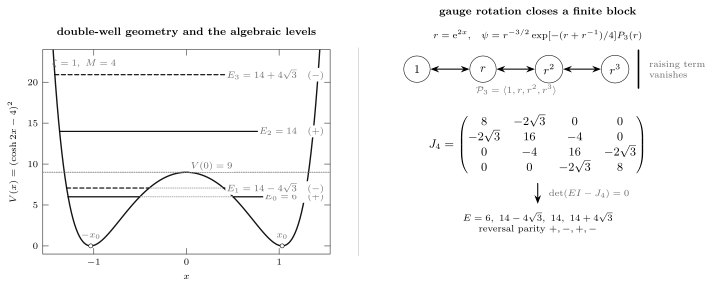
One parameter choice displays both structures. The left panel shows two sub-barrier algebraic states and two algebraic states above the barrier. The right panel shows why exactly four energies are algebraic: $\mathcal P_3$ is invariant and its finite Jacobi matrix has reversal parities $+,-,+,-$.

Reflection folding changes DCHE into CHE

The same Razavy equation also has a confluent-Heun realization. This is not a competing classification. The coordinate

$$t=\sinh^2x$$

quotients the reflection $x\sim-x$: both spatial infinities map to $t=\infty$, while the origin becomes a finite regular singular point.

Expert checkpoint: the four parity-folded CHE sectors

Let $p,c\in\{0,1\}$ and set

$$\psi(x) = \ee^{-\zeta\cosh 2x/2} (\sinh x)^p(\cosh x)^cY(t).$$

The exponent $p$ fixes physical parity. Direct substitution gives

$$\begin{aligned} t(t+1)Y'' &+ \left[ p+\frac12 +(p+c+1-2\zeta)t -2\zeta t^2 \right]Y' \\ &+ \left[ d_0+\zeta(M-p-c-1)t \right]Y =0, \end{aligned}$$

where

$$d_0 = \frac{E-M^2-\zeta^2}{4} + \frac{\zeta}{2}(M-1-2p) + \frac{p+c+2pc}{4}.$$

With $s=-t$, this is the DLMF CHE with

$$\begin{aligned} \epsilon_{\mathrm C}&=2\zeta, & \gamma_{\mathrm C}&=p+\frac12, \\ \delta_{\mathrm C}&=c+\frac12, & \alpha_{\mathrm C}&=-2\zeta N, & q_{\mathrm C}&=-d_0, \end{aligned}$$

provided

$$M=2N+p+c+1.$$

Thus $\alpha_{\mathrm C}=-N\epsilon_{\mathrm C}$, exactly the CHE polynomial-wall condition. The available sectors are

$M$	Parity	$(p,c)$	Degree
$2K+1$	even	$(0,0)$	$N=K$
$2K+1$	odd	$(1,1)$	$N=K-1$
$2K$	even	$(0,1)$	$N=K-1$
$2K$	odd	$(1,0)$	$N=K-1$

Rows with $N<0$ are absent. In particular, $M=1$ has only the even sector $(p,c,N)=(0,0,0)$.

Their dimensions add to $M$. The unquotiented $r$-plane has two irregular ends and is DCHE; the reflection quotient has two finite regular points and one irregular infinity and is CHE.

Analytic continuation $x=i\theta$ gives the periodic Whittaker–Hill operator

$$H_{\mathrm{WH}} = -\frac{\dd^2}{\dd\theta^2} - \bigl(\zeta\cos 2\theta-M\bigr)^2$$

and reverses the algebraic energies, $E_{\mathrm{WH}}=-E$. This anti-isospectral map explains the finite trigonometric solutions, but it does not identify the complete spectra: square integrability on $\mathbb R$ and periodic or antiperiodic boundary conditions on a circle are different global problems.

Finite algebra and the full spectrum agree where they overlap

The companion program razavy-qes-spectrum.py uses two independent representations:

1. the exact $M\times M$ Jacobi block;
2. a centered finite-interval approximation to the real-line operator, reduced by parity, solved by Sturm bisection, and Richardson extrapolated after step halving.

Run

python3 public/code/advanced-ode/razavy-qes-spectrum.py
python3 public/code/advanced-ode/razavy-qes-spectrum.py \
  --mode high --csv /tmp/razavy-spectrum.csv

The high profile means a finer grid, not a guarantee that every last floating-point digit improves monotonically. Compare its refinement shifts with the default profile; neither run is a certified enclosure.

The default $\zeta=1$, $M=4$ audit gives

$n$	Parity	Finite block	Real-line Richardson	Status
0	even	$6.000000000000$	$6.000000000136$	algebraic
1	odd	$7.071796769724$	$7.071796769878$	algebraic
2	even	$14.000000000000$	$14.000000000175$	algebraic
3	odd	$20.928203230276$	$20.928203230045$	algebraic
4	even	—	$29.86344328$	nonalgebraic

The maximum finite-block/direct gap over the four algebraic levels is $2.31\times10^{-10}$. The maximum fine-grid-to-Richardson shift within that sector is $2.06\times10^{-5}$; the larger printed levels are also mesh-refined and reported separately. The finite matrix commutes with reversal to floating-point zero.

The fifth row is the decisive negative control. The physical operator has not run out of states; only the invariant polynomial block has ended. Likewise, if one detunes an integer $m$ to $M=m+\Delta$ and tries to retain $\mathcal P_{m-1}$, then

$$\mathcal H_g r^{m-1} = -2\zeta\Delta\,r^m + \text{terms in }\mathcal P_{m-1}.$$

Any $\Delta\ne0$ leaks through the supposed termination wall. The connection determinant and exact-WKB cycles remain meaningful, but the finite characteristic polynomial does not.

What remains exact away from the algebraic slice

Statement	Integer $M$	Noninteger $M$
Self-adjoint, confining real-line problem	yes	yes
Even/odd connection determinant	yes	yes
DCHE reduction on the negative ray	yes	yes
Finite invariant polynomial space	yes	no
First $M$ levels from $\Pi_M$	yes	not defined
Exact-WKB turning-point problem	yes	yes

QES is therefore an exact calibration surface inside a larger analytic family. It neither makes the WKB series terminate nor replaces the connection problem for higher levels. That distinction is the starting point for the later comparison of quasi-exact solvability with generic exact-WKB behavior.

The finite block and the direct coordinate grid established here will also serve as two baselines in the chapter capstone; exact WKB supplies the third.

Common pitfalls

Equating “double well” with “QES.” The first condition is the open inequality $M>\zeta$; the second is the discrete condition $M\in\mathbb N$. Either can hold without the other.

Stopping after the integer condition. Integer $M$ closes $\mathcal P_{M-1}$, but an energy is selected only after $\Pi_M(E)=0$. Closure and finite compatibility are separate tests.

Calling every Razavy equation CHE or every one DCHE. The one-to-one exponential coordinate preserves two irregular ends and gives DCHE. The reflection quotient folds those ends together and gives CHE.

Extending anti-isospectrality to the full spectrum. Analytic continuation matches the finite algebraic solutions. It does not equate real-line decay with periodic or antiperiodic boundary conditions.

Exercises

1. Recover the historical normalization

Starting from $(\zeta\cosh2x-M)^2$, use $\cosh^2 2x=(1+\cosh4x)/2$ to derive $V_{\mathrm R}$ and the energy shift.

Solution

Expanding gives

$$\begin{aligned} \bigl(\zeta\cosh2x-M\bigr)^2 ={}& \frac{\zeta^2}{2}\cosh4x -2M\zeta\cosh2x \\ &+ M^2+\frac{\zeta^2}{2}. \end{aligned}$$

Set $\xi=2\zeta$ and $M=n+1$. Subtracting $M^2+\zeta^2$ leaves

$$\frac{\xi^2}{8}(\cosh4x-1)-M\xi\cosh2x.$$

Therefore $E=\epsilon+M^2+\zeta^2$.

2. Classify the geometry and compute the bottom action

Find all real critical points, classify the case $M=\zeta$, and evaluate $S_0$ in the double-well chamber.

Solution

The critical equation is

$$\sinh2x\,(\zeta\cosh2x-M)=0.$$

If $M>\zeta$, the second factor gives $x=\pm x_0$ with $x_0=\tfrac12\operatorname{arcosh}(M/\zeta)$; these are minima, while $x=0$ is a maximum. If $M<\zeta$, only $x=0$ is real and it is a minimum. At equality,

$$V=M^2(\cosh2x-1)^2=4M^2x^4+O(x^6).$$

Finally,

$$\begin{aligned} S_0 &= 2\int_0^{x_0}(M-\zeta\cosh2x)\,\dd x \\ &= 2Mx_0-\zeta\sinh2x_0 \\ &= M\operatorname{arcosh}\!\left(\frac M\zeta\right) -\sqrt{M^2-\zeta^2}. \end{aligned}$$

3. Verify the DCHE passport

Carry out the changes $r=\ee^{2x}$ and $\rho=-\zeta r/2$, including the full gauge, and recover the four DLMF parameters.

Solution

Since

$$\frac{\dd}{\dd x}=2r\frac{\dd}{\dd r}, \qquad \frac{\dd^2}{\dd x^2} = 4r^2\frac{\dd^2}{\dd r^2} +4r\frac{\dd}{\dd r},$$

and $\cosh2x=(r+r^{-1})/2$, direct substitution yields the displayed $r$-equation. Factoring

$$r^{(1-M)/2} \exp\!\left[-\frac{\zeta}{4}(r+r^{-1})\right]$$

and using $\rho=-\zeta r/2$ gives

$$Y'' + \left( 1+\frac{2-M}{\rho} -\frac{\zeta^2}{4\rho^2} \right)Y' + \frac{(1-M)\rho-(\zeta^2+2M-1-E)/4}{\rho^2}Y =0.$$

Reading against the DLMF form gives the stated tuple.

4. Derive both termination conditions

Apply $\mathcal H_g$ to $r^k$, derive the recurrence for $\Pi_k$, and show why $M\in\mathbb N$ alone does not select an energy.

Solution

The gauged operator acts by

$$\begin{aligned} \mathcal H_g r^k ={}& b_k r^k -2\zeta k\,r^{k-1} \\ &+ 2\zeta(k-M+1)r^{k+1}. \end{aligned}$$

The raising coefficient vanishes at $k=M-1$, so $\mathcal P_{M-1}$ is invariant when $M$ is a positive integer. Equating successive coefficients with

$$c_k = \frac{(-1)^k\Pi_k(E)}{(2\zeta)^k k!}$$

gives

$$\Pi_{k+1} =(E-b_k)\Pi_k -4\zeta^2k(M-k)\Pi_{k-1}.$$

The last coefficient vanishes only when $\Pi_M(E)=0$. Thus invariance selects the finite space, while the degree-$M$ equation selects the allowed energies.

5. Solve the first two nontrivial sectors

Find the algebraic energies and parities for $M=2$ and $M=3$.

Solution

For $M=2$,

$$J_2 = \begin{pmatrix} \zeta^2+3&-2\zeta\\ -2\zeta&\zeta^2+3 \end{pmatrix}.$$

Hence

$$\begin{aligned} E_0&=\zeta^2+3-2\zeta, & \psi_0&\propto \ee^{-\zeta\cosh2x/2}\cosh x, \\ E_1&=\zeta^2+3+2\zeta, & \psi_1&\propto \ee^{-\zeta\cosh2x/2}\sinh x. \end{aligned}$$

For $M=3$, put $R=\sqrt{1+4\zeta^2}$. The three levels are

$$E_0=\zeta^2+7-2R, \qquad E_1=\zeta^2+5, \qquad E_2=\zeta^2+7+2R.$$

The middle state is odd,

$$\psi_1\propto \ee^{-\zeta\cosh2x/2}\sinh2x,$$

while the lower and upper states are even and proportional to

$$\ee^{-\zeta\cosh2x/2} \left[ 2\zeta+(1\pm R)\cosh2x \right],$$

with the plus sign for $E_0$ and the minus sign for $E_2$.

6. Count the parity-folded sectors

Starting from $M=2N+p+c+1$, recover the number of even and odd algebraic states for even and odd $M$.

Solution

If $M=2K+1$ with $K\ge1$, the even choice $(p,c)=(0,0)$ has $N=K$ and dimension $K+1$, while the odd choice $(1,1)$ has $N=K-1$ and dimension $K$. For $K=0$, only the one-dimensional even sector remains.

If $M=2K$, the even choice $(0,1)$ and odd choice $(1,0)$ both have $N=K-1$. Each sector has dimension $K$, for a total of $2K=M$.

7. Expose a false finite cutoff

Let the physical parameter be $M=m+\Delta$ with $m\in\mathbb N$. Compute the coefficient outside $\mathcal P_{m-1}$ when $\mathcal H_g$ acts on its top monomial.

Solution

The $r^m$ term receives $2\zeta(m-1)r^m$ from $2\zeta r^2\partial_r$ and $-2\zeta(M-1)r^m$ from the multiplication term. Their sum is

$$2\zeta(m-M)r^m=-2\zeta\Delta\,r^m.$$

It vanishes only at $\Delta=0$. A numerical $m\times m$ cutoff at nonzero $\Delta$ is a finite-section approximation, not exact QES termination.

8. Audit the algebraic and nonalgebraic levels

Run the companion program at its default settings. Verify the parity order, the four exact roots, and the existence of the fifth state.

Solution

The finite matrix gives

$$6,\quad 14-4\sqrt3,\quad 14,\quad 14+4\sqrt3$$

with reversal parity $+,-,+,-$. The refined coordinate calculation agrees with all four to better than $2.4\times10^{-10}$ in the default run. It also returns

$$E_4\approx29.86344328,$$

an even state for which the finite algebraic column is absent. This fifth level is not a numerical defect; it is the first state beyond the exact $M=4$ sector.

References

• M. Razavy, “An exactly soluble Schrödinger equation with a bistable potential,” American Journal of Physics 48 (4) (1980), 285–288, doi:10.1119/1.12141. This is the original potential, finite hyperbolic ansatz, and low-state construction.
• F. Finkel, A. González-López, and M. A. Rodríguez, “On the families of orthogonal polynomials associated to the Razavy potential,” Journal of Physics A: Mathematical and General 32 (39) (1999), 6821–6835, doi:10.1088/0305-4470/32/39/308, arXiv:math-ph/9905020. This supplies the square convention, hidden-$\mathfrak{sl}_2$ algebraization, and energy-polynomial recurrence.
• NIST Digital Library of Mathematical Functions, §31.12, Confluent Forms of Heun’s Equation, fixes the conventions used here through equation 31.12.1 for CHE and equation 31.12.2 for DCHE.
• A. V. Turbiner, “Quasi-exactly-solvable problems and $sl(2)$ algebra,” Communications in Mathematical Physics 118 (3) (1988), 467–474, doi:10.1007/BF01466727, gives the invariant-space framework for one-dimensional QES operators.
• A. González-López, N. Kamran, and P. J. Olver, “Normalizability of one-dimensional quasi-exactly solvable Schrödinger operators,” Communications in Mathematical Physics 153 (1) (1993), 117–146, doi:10.1007/BF02099042, separates formal algebraization from physical admissibility.
• S. Becker, M. Mirahmadi, B. Schmidt, K. Schatz, and B. Friedrich, “Conditional quasi-exact solvability of the quantum planar pendulum and of its anti-isospectral hyperbolic counterpart,” The European Physical Journal D 71 (2017), 149, doi:10.1140/epjd/e2017-80134-6, arXiv:1702.08733, develops the parity sectors and the finite anti-isospectral correspondence.