Borel–Padé Computation and High-Precision Spectral Tests

Exact WKB becomes computational only after several analytic choices have already been made. A finite list of WKB coefficients is not a Borel sum; a rational function fitted to that list is not the exact Borel transform; and a small determinant residual is not a certified eigenvalue. The numerical task is to preserve those distinctions while turning the declared exact-WKB passport into reproducible numbers.

This page builds that workflow around two exact laboratories. The regularized Weber path isolates the Borel–Padé problem because its Borel-pole lattice, positive-ray sum, and lateral jump are known in closed form. The PT-symmetric Airy box isolates the spectral problem because its exact determinant can be compared with an unrelated arbitrary-precision Taylor shooting calculation. Together they test the two halves of the workflow without pretending to be one end-to-end spectral calculation or a general convergence theorem. In particular, the Airy roots are not produced from the Weber Borel data.

The computational contract

For a new end-to-end problem, a spectral digit should be reported only after the relevant coefficient order, Padé shape, working precision, quadrature contour, lateral offset, ODE discretization, contour mesh, and root refinement have been varied, and after an independent representation agrees. The two exact laboratories below are deliberately half-pipeline calibrations: Weber audits coefficient order, Padé algebra, poles, rays, and lateral offset; Airy audits two determinants, two Taylor discretizations, node doubling, and an independent $D_E/D$ contour integral.

The core pipeline is

$$\begin{gathered} \text{WKB coefficients} \longrightarrow \text{Borel germ}, \\ \text{Padé continuation} \longrightarrow \text{directional Laplace integral}, \\ \text{Voros symbols} \longrightarrow \text{boundary determinant}, \\ \text{root count} \longrightarrow \text{polished and cross-checked zeros}. \end{gathered}$$

Status ledger

Claim or computation	Status
Padé coefficient matching through degree $L+M$	Exact algebra for the supplied coefficients
Finite WKB coefficients equal the intended formal series	Exact only after the recurrence, cycles, and regularization have been audited
A finite Padé approximant is the analytic continuation	False; it is a numerical model of that continuation
Stable Padé poles locate Borel singularities	Numerical evidence; exact only in a calibrated meromorphic example or under an applicable theorem
A pole string represents a branch cut	An interpretation supported by order and shape stability, not an identity at finite order
Quadrature of a fixed rational integrand	Numerically controllable, and certifiable with explicit bounds
Finite-order Padé continuation error	No universal a posteriori bound
Weber pole lattice, gamma sum, and lateral jump	Exact benchmark identities
Argument-principle root count	Exact for a nonvanishing contour; a sampled winding needs a numerical error audit
Airy determinant and Taylor-shooting agreement	Independent high-precision cross-verification
High precision by itself is certification	False; rigorous certification needs enclosures such as ball or interval bounds

Finite coefficients do not yet define a sum

Four objects that are often called “the Borel transform” must be kept separate:

Layer	Object	What is known
Formal tail	$\widehat f-a_0$	Coefficients generated algebraically
Borel germ	$\mathcal B\widehat f$ near $\xi=0$	A finite Taylor list, or an actual convergent germ under a Gevrey bound
Rational continuation	$R_{L,M}=P_L/Q_M$	A finite Padé approximation fixed by coefficient matching
Directional value	$a_0+\mathcal L_\theta R_{L,M}$	A numerical approximation to a declared Borel sum

The final spectrum adds two further layers: resummed symbols must be inserted into the complete boundary determinant, and the zeros of that determinant must be counted and refined. Skipping a layer can produce a beautifully converged answer to a different problem.

The evidence vocabulary from Chapter 4’s verified-numerics page is useful here:

• computed means that one finite prescription returned a value;
• internally converged means that controlled refinements agree;
• cross-verified means that a representation with different failure modes agrees;
• certified means that the relevant value, integral, or zero lies in a proved enclosure; and
• physically validated additionally checks the boundary and sheet interpretation.

Borel–Padé calculations with arbitrary precision commonly reach the first three levels. They reach certification only when the continuation, quadrature, and zero-count errors have genuine bounds.

Implement the shifted transform exactly once

Page 1 fixed the normalization

$$\widehat f(\hbar) = a_0+\sum_{n\geq1}a_n\hbar^n, \qquad \mathcal B\widehat f(\xi) = \sum_{j\geq0} \frac{a_{j+1}}{j!}\xi^j.$$

Given $N+1$ Borel coefficients $b_0,\ldots,b_N$, choose $L+M=N$ and write

$$\begin{aligned} P_L(\xi) &= \sum_{r=0}^{L}p_r\xi^r, \\ Q_M(\xi) &= 1+\sum_{s=1}^{M}q_s\xi^s. \end{aligned}$$

The $[L/M]$ Padé approximant is defined by

$$Q_M(\xi) \sum_{n=0}^{N}b_n\xi^n - P_L(\xi) = O(\xi^{N+1}).$$

The denominator coefficients solve the square system

$$\sum_{s=1}^{M} q_s b_{n-s} = -b_n, \qquad n=L+1,\ldots,L+M,$$

where coefficients with negative indices are zero. The numerator then follows from

$$p_n = \sum_{s=0}^{\min(M,n)} q_s b_{n-s}, \qquad q_0=1.$$

This calculation should be done exactly when the input coefficients are exact rationals. For numerical input it should be repeated at guard precision. A singular system is a defective Padé type, not an invitation to hide the problem with an unreported least-squares solve.

Quantum periods have two different factorial shifts

For an even-$\hbar$ quantum period,

$$\widehat\Pi_\gamma = \Pi_{\gamma,0} + \sum_{k\geq1} \Pi_{\gamma,2k}\hbar^{2k},$$

the period tail and the quantum part of the Voros exponent are

$$\begin{aligned} \widehat\Pi_\gamma-\Pi_{\gamma,0} &= \sum_{k\geq1} \Pi_{\gamma,2k}\hbar^{2k}, \\ \widehat V_\gamma^{\mathrm q} &= \frac{ \widehat\Pi_\gamma-\Pi_{\gamma,0} }{\hbar} = \sum_{k\geq1} \Pi_{\gamma,2k}\hbar^{2k-1}. \end{aligned}$$

Their shifted Borel transforms are therefore

$$\begin{aligned} \mathcal B \left( \widehat\Pi_\gamma-\Pi_{\gamma,0} \right) &= \sum_{k\geq1} \Pi_{\gamma,2k} \frac{\xi^{2k-1}}{(2k-1)!}, \\ \mathcal B\widehat V_\gamma^{\mathrm q} &= \sum_{k\geq1} \Pi_{\gamma,2k} \frac{\xi^{2k-2}}{(2k-2)!}. \end{aligned}$$

Using the first transform in place of the second produces

$$\mathcal B_{\mathrm{wrong}}(\xi) = \frac{1}{\xi} \int_0^\xi \mathcal B\widehat V_\gamma^{\mathrm q}(s) \,\dd s.$$

The Laplace inverse still reconstructs the power $\hbar^{2k-1}$, but divides its coefficient by $2k-1$.

Four implementation rules prevent the most expensive mistakes:

1. Factor $\exp(Z_\gamma/\hbar)$ before applying the ordinary Borel transform.
2. Retain the zero odd or even coefficients in a generic series. A substitution such as $u=\xi^2$ is safe only when parity is proved.
3. Generate coefficients exactly or at their true working precision. Promoting binary64 inputs to 100 digits restores no information.
4. Rescale $\xi=A_{\mathrm{scale}}u$ when a known nearest action is far from unit scale, and record that scale with the output.

A Padé table is an audit, not a decoration

One diagonal approximant cannot reveal whether its apparent poles are stable. At fixed coefficient order, inspect several near-diagonal shapes, for example

$$L-M\in\{-2,-1,0,1,2\}, \qquad L+M\leq N.$$

Repeat the table as $N$ and the arithmetic precision increase. The pole and zero maps then have three common signatures:

Observed pattern	Plausible interpretation	Required check
An isolated pole and residue stabilize	Meromorphic Borel singularity	Vary $N$, shape, precision, and scaling
Alternating pole–zero strings stabilize collectively	Rational approximation to a branch cut	Compare the whole string, not individual poles
A close pole–zero pair moves rapidly	Froissart doublet or coefficient noise	Track it across the full Padé table

A convenient scale-invariant doublet diagnostic for a denominator pole $p\neq0$ is

$$d_{\mathrm F}(p) := \min_{P_L(z)=0} \frac{|p-z|}{\max(|p|,|z|)}.$$

A denominator zero cannot occur at $p=0$ because $Q_M(0)=1$, and this ratio is unchanged by a common nonzero rescaling of the Borel coordinate. Flagging a small $d_{\mathrm F}$ is useful; silently cancelling the pair is not. Cancellation can change the analytic dependence on $E$ and invalidate a later argument-principle calculation.

Withheld-coefficient prediction provides another independent axis. Construct $R_{L,M}$ without the last few known coefficients, re-expand it, and compare the predictions with the withheld values. Good prediction does not prove global continuation, but bad prediction is an immediate failure.

General Padé convergence theorems have hypotheses. Stahl-type results, for example, concern convergence in capacity for specified multivalued analytic functions. They do not guarantee uniform convergence along an arbitrary Laplace ray for every resurgent germ.

The Laplace contour is part of the answer

For a pole-free ray $\xi=\ee^{\ii\phi}t$, the shifted Borel–Padé approximation is

$$\mathcal S_{\phi}^{[L/M]}\widehat f(\hbar) = a_0 + \ee^{\ii\phi} \int_0^\infty \exp\!\left( -\frac{\ee^{\ii\phi}t}{\hbar} \right) R_{L,M}(\ee^{\ii\phi}t) \,\dd t.$$

There is no factor $1/\hbar$. If the continued Borel transform obeys an upper bound proportional to $\exp(\kappa t)$ along the ray, absolute convergence follows from the sufficient condition

$$\sigma := \operatorname{Re} \left( \frac{\ee^{\ii\phi}}{\hbar} \right) > \kappa.$$

For a singular central direction $\theta_0$, this chapter uses

$$\theta_+ = \theta_0+\delta, \qquad \theta_- = \theta_0-\delta, \qquad \delta>0,$$

and

$$\operatorname{Disc}_{\theta_0} = \mathcal S_{\theta_0+} - \mathcal S_{\theta_0-}.$$

A fixed offset represents the intended lateral homotopy class only if the rotated ray can be deformed to that lateral contour without crossing another singularity. Varying $\delta$ tests numerical clearance from Padé poles; it does not replace the homotopy argument.

Tail error and continuation error are different quantities

Suppose that for $t\geq T$,

$$\left| R_{L,M}(\ee^{\ii\phi}t) \right| \leq C(1+t)^p\ee^{\kappa t}, \qquad \tau:=\sigma-\kappa>0.$$

Then the omitted tail is bounded by

$$\begin{aligned} \left| \int_T^\infty \ee^{-\ee^{\ii\phi}t/\hbar} R_{L,M}(\ee^{\ii\phi}t) \,\dd t \right| &\leq C\int_T^\infty \ee^{-\tau t}(1+t)^p \,\dd t \\ &= C\ee^\tau \tau^{-p-1} \Gamma\!\left( p+1,\tau(1+T) \right). \end{aligned}$$

This controls the tail of the rational approximation. It says nothing about the difference between that rational function and the exact continued Borel transform. If an independent bound

$$\left| \mathcal B\widehat f(\ee^{\ii\phi}t) - R_{L,M}(\ee^{\ii\phi}t) \right| \leq \varepsilon(t)$$

is available, integrate $\varepsilon(t)$ against the same Laplace kernel. Without it, Padé-order stability remains evidence rather than an enclosure.

A principal-value integral is not a substitute for two lateral sums. Likewise, a median resummation is fixed by the transseries and Stokes automorphism of Page 7; it is not generically the arithmetic mean of two numerical laterals.

Weber exposes the whole Borel–Padé mechanism

Page 5 introduced the regularized Weber exponent

$$\widehat W_{\mathrm W}(\hbar) = \sum_{k\geq1} \frac{ \left(2^{1-2k}-1\right)B_{2k} }{ 2k(2k-1)\mu^{2k-1} } \hbar^{2k-1}.$$

Its shifted Borel transform is known exactly:

$$\mathcal B\widehat W_{\mathrm W}(\xi) = \frac{1}{2\xi} \left[ \operatorname{csch} \left( \frac{\xi}{2\mu} \right) - \frac{2\mu}{\xi} \right].$$

The origin is removable. The nonzero poles and residues are

$$\begin{aligned} \xi_k &= 2\pi\ii\mu k, \\ \operatorname*{Res}_{\xi=\xi_k} \mathcal B\widehat W_{\mathrm W} &= \frac{(-1)^k}{2\pi\ii k}, \qquad k\in\mathbb Z\setminus\{0\}. \end{aligned}$$

Because this Borel transform is provably even, set $u=\xi^2$ and use

$$G_K(u) = \sum_{r=0}^{K-1}c_ru^r, \qquad c_r = \frac{ \left(2^{-2r-1}-1\right)B_{2r+2} }{ (2r+2)!\,\mu^{2r+1} }.$$

Choose

$$L = \left\lceil\frac{K-1}{2}\right\rceil, \qquad M = \left\lfloor\frac{K-1}{2}\right\rfloor,$$

construct $P_L(u)/Q_M(u)$ exactly, and evaluate

$$R_K(\xi) = \frac{P_L(\xi^2)}{Q_M(\xi^2)}.$$

The parity reduction is specific to this audited symmetry. Applying it to a generic Borel germ can identify the $+\xi$ and $-\xi$ directions incorrectly.

The nonsingular ray tests continuation and quadrature

Take

$$\mu=1, \qquad \hbar=0.2, \qquad t=\frac{\mu}{\hbar}=5.$$

The exact positive-ray sum should be evaluated in logarithmic form:

$$W_{\mathrm{exact}} = t + \log\Gamma\!\left(t+\frac12\right) - \frac12\log(2\pi) - t\log t.$$

Numerically,

$$W_{\mathrm{exact}} = -0.008314127756458320906725546713964838938099753 \ldots.$$

With 80-decimal arithmetic, exact Bernoulli input, and split high-precision quadrature, the companion checker obtains

$K$	Padé type in $u$	Absolute error
4	$[2/1]$	$2.8490\times10^{-12}$
8	$[4/3]$	$1.4897\times10^{-21}$
12	$[6/5]$	$1.2273\times10^{-30}$
20	$[10/9]$	$1.1536\times10^{-48}$

The table is unusually clean because the target is meromorphic and exactly known. It calibrates the code; it does not promise the same rate for a Borel transform with cuts or several competing actions.

Rotated rays fix the lateral sign

Now set

$$\hbar=\ii, \qquad \theta_0=\frac{\pi}{2}, \qquad \theta_\pm=\frac{\pi}{2}\pm0.1.$$

Both rotated Laplace kernels decay because

$$\operatorname{Re} \left( \frac{\ee^{\ii\theta_\pm}}{\ii} \right) = \cos(0.1)>0.$$

The closest point on either rotated ray to $\xi_k=2\pi\ii k$ occurs at $t=2\pi k\cos(0.1)$. The implementation splits at the nearby action scales $t=2\pi k$; these breakpoints resolve the narrow features without being claimed as the exact projections. The resulting difference is

$$\begin{aligned} \mathcal S_{\theta_0+}\widehat W_{\mathrm W} - \mathcal S_{\theta_0-}\widehat W_{\mathrm W} &= \log\!\left(1+\ee^{-2\pi}\right) \\ &= 0.00186570122829807564414623197325513 \ldots. \end{aligned}$$

The $K=8$ and $K=16$ Padé calculations miss this value by $2.34\times10^{-10}$ and $6.86\times10^{-18}$, respectively. The positive sign is therefore checked simultaneously by the Borel residues, the rotated quadrature, and Page 5’s DDP convention.

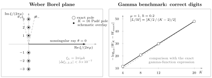
Borel–Padé continuation must be audited in both the Borel plane and the final observable. Left: open circles are the exact Weber poles $\xi_k=2\pi\ii\mu k$; filled symbols schematically overlay the computed $K=16$ Padé poles, whose first three absolute displacements are approximately $3.73\times10^{-23}$, $6.42\times10^{-13}$, and $2.91\times10^{-7}$ at the plot’s scale. The positive and lateral Laplace rays remain explicit. Right: comparison with the exact gamma-function expression shows nearly linear growth of benchmark-correct digits with the number $K$ of nonzero coefficients in this meromorphic calibration.

Resummed exponents must enter the complete determinant

For each required cycle or relative path, restore the classical action only after summing the quantum correction:

$$\mathcal V_{\gamma,\phi}^{\mathrm{BP}} = \exp\!\left[ \frac{Z_\gamma}{\hbar} + \mathcal S_\phi^{\mathrm{BP}} \widehat V_\gamma^{\mathrm q} \right].$$

Then insert all symbols into the chamber-correct route product from Page 6. A single period equation detached from its endpoint lines is not a boundary determinant. When the Stokes graph changes, transform every symbol, path, and endpoint line together.

The raw exponentials can overflow or underflow long before the determinant loses information. Work with logarithmic symbols and scaled endpoint frames. If the canonical columns are rescaled by analytic nonzero functions,

$$c_L\longmapsto f_L(E)c_L, \qquad c_R\longmapsto f_R(E)c_R,$$

then

$$D(E) = \det(c_L,c_R) \longmapsto f_L(E)f_R(E)D(E).$$

The zero divisor and its multiplicities are unchanged. Record the scale factors anyway: values of two differently normalized determinants cannot be compared pointwise without them.

A phase-unwrapped logarithmic quantization condition is useful for initial guesses. Final roots should solve a single-valued determinant. Changing a numerical branch of $\log\mathcal V_\gamma$ can otherwise look like changing the quantum number.

Count roots before polishing them

Let $D(E)$ be holomorphic inside and nonzero on a positively oriented contour $C$. The argument principle and its moments give

$$s_k := \frac{1}{2\pi\ii} \oint_C E^k\frac{D_E(E)}{D(E)} \,\dd E = \sum_j m_jE_j^k.$$

In particular, $s_0$ counts enclosed zeros with multiplicity. If the chosen characteristic function is meromorphic, the same integral counts zeros minus poles; known normalization poles must be removed or counted explicitly.

A derivative-free first pass samples $D$ at ordered contour nodes:

$$N_h = \frac{1}{2\pi} \sum_j \operatorname{Arg} \left( \frac{D(E_{j+1})}{D(E_j)} \right).$$

Insert midpoints whenever an image segment approaches the origin or a phase increment becomes large. Then double the node count and compare with a separate quadrature of $D_E/D$. An integer-looking phase sum is not certified unless nonvanishing on the whole contour and evaluation errors are controlled.

For two enclosed zeros and no poles,

$$c=\frac{s_1}{2}, \qquad d^2=\frac{s_2}{2}-c^2, \qquad E_\pm=c\pm d.$$

The moments give root guesses without independent Newton seeds. They also show why $s_0=2$ cannot distinguish two close simple roots from one double root: at a double root $d^2=0$, but one must additionally check

$$D=0, \qquad D_E=0, \qquad D_{EE}\neq0.$$

Along a simple spectral branch depending on $\lambda$,

$$\frac{\dd E}{\dd\lambda} = - \frac{D_\lambda}{D_E}.$$

Use this as a predictor and correct with the single-valued determinant. When $|D_E|$ collapses, stop simple-root tracking and solve the augmented system $D=D_E=0$ or change to a Puiseux or pseudo-arclength parameter.

If a computable approximation $\widetilde D$ obeys

$$\sup_C|D-\widetilde D| < \inf_C|\widetilde D|,$$

Rouché’s theorem transfers the zero count. Chapter 4 develops the corresponding Rouché and Krawczyk enclosures; this page uses the argument principle as a high-precision diagnostic rather than claiming an interval proof.

The Airy box supplies an independent spectral audit

Return to Page 8’s problem

$$-\psi''+\ii gx\psi=E\psi, \qquad \psi(-1)=\psi(1)=0.$$

With

$$\alpha=g^{1/3}\ee^{\ii\pi/6}, \qquad z_\pm = \alpha \left( \pm1+\frac{\ii E}{g} \right),$$

the raw and PT-real-normalized determinants are

$$\begin{aligned} D_{\mathrm A}(E,g) &= \operatorname{Ai}(z_-)\operatorname{Bi}(z_+) - \operatorname{Ai}(z_+)\operatorname{Bi}(z_-), \\ \Delta_{\mathrm A}(E,g) &= \ee^{-\ii\pi/6}D_{\mathrm A}(E,g). \end{aligned}$$

Special-function evaluation alone is not an independent check. Instead, shoot the ODE from

$$y(-1)=0, \qquad y'(-1)=1,$$

and define $F(E,g)=y(1)$. Around a Taylor center $x_0$, write

$$y(x_0+s) = \sum_{n\geq0}c_ns^n.$$

The differential equation gives the exact recurrence

$$c_{n+2} = \frac{ (\ii gx_0-E)c_n+\ii g c_{n-1} }{ (n+2)(n+1) }, \qquad c_{-1}=0.$$

Marching this recurrence over several equal subintervals uses only polynomial arithmetic at arbitrary precision. It shares neither Airy special-function algorithms nor a finite-difference eigensolver with $\Delta_{\mathrm A}$.

The determinant normalization is exact

The Airy Wronskian is

$$\operatorname{Ai}(z)\operatorname{Bi}'(z) - \operatorname{Ai}'(z)\operatorname{Bi}(z) = \frac1\pi.$$

Consequently,

$$y(x) = \frac{\pi}{\alpha} \left[ \operatorname{Ai}(z_-)\operatorname{Bi}(z(x)) - \operatorname{Bi}(z_-)\operatorname{Ai}(z(x)) \right]$$

has the declared initial data, and hence

$$F(E,g) = \frac{\pi}{\alpha}D_{\mathrm A}(E,g) = \frac{\pi}{g^{1/3}}\Delta_{\mathrm A}(E,g).$$

This zero-free normalization identity checks the Airy determinant’s phase as well as its zero set.

At $g=10$, 75-decimal arithmetic, eight Taylor steps, and order 60 give

Quantity	High-precision value or result
First zero	$4.578490418291691965603794\ldots$
Second zero	$8.996683255712348208437330\ldots$
Airy versus Taylor-shooting roots	Agreement better than $2\times10^{-58}$; a second Taylor grid agrees beyond $10^{-54}$
Rectangle $3\leq\operatorname{Re}E\leq10$, $	\operatorname{Im}E
Minimum sampled $	\Delta_{\mathrm A}

The mutually agreeing numerical counts are consistent with exactly the two displayed roots in the box. The largest adjacent phase increments fall from $0.092396216\ldots$ to $0.046211656\ldots$ when the edge mesh is doubled. The sampled clearance is a useful safety diagnostic, but not a lower bound between samples.

Near the first exceptional point,

$$\begin{aligned} g_c &= 12.31245567226052505295708367\ldots, \\ E_c &= 7.108599596764948797243418965\ldots, \end{aligned}$$

the count remains two while $D_E$ tends to zero. Ordinary Newton conditioning therefore deteriorates even though the contour count is stable. The augmented equations and the nonzero derivatives $D_{EE}$ and $D_g$ distinguish the double zero from two numerically unresolved simple zeros.

Cross-verification is not certification

The Airy and Taylor determinants agree to far more digits than are printed; two Taylor grids agree; and node doubling agrees with a separate $D_E/D$ contour integral. This is strong cross-verification. A certified count would additionally enclose the Taylor remainder, special-function evaluations, and contour nonvanishing—tasks suited to ball arithmetic.

A refinement tensor exposes the error floor

Record the numerical prescription as a tuple rather than a single “precision”:

$$\mathfrak R = \left( K,L,M,p_{\mathrm{work}}, \phi,\delta,T, \varepsilon_{\mathrm{quad}}, \varepsilon_{\mathrm{root}}, n_x,N_x \right).$$

Here $K$ is the coefficient count, $p_{\mathrm{work}}$ the arithmetic precision, $(n_x,N_x)$ the number and order of Taylor steps, and the remaining entries describe the rational approximation, contour, quadrature, and root solve.

Refinement axis	Primary failure mode exposed
$K$	Insufficient formal or Borel information
$L,M$	Dependence on rational-continuation shape
$p_{\mathrm{work}}$	Padé-system conditioning and roundoff
$\phi,\delta$	Wrong ray, lateral class, or poor pole clearance
$T,\varepsilon_{\mathrm{quad}}$	Tail truncation and quadrature
Root tolerance and contour nodes	Missed roots or incomplete polishing
$n_x,N_x$ or match point	Independent ODE propagation error

Vary one axis at a time. If every entry is changed simultaneously, an improved result gives no information about which error was dominant.

At a fixed spectral parameter $E$, the schematic determinant-evaluation decomposition

$$\begin{aligned} D-\widetilde D ={}& \left(D-D_{K,L,M}^{\mathrm{BP}}\right) \\ &+ \left( D_{K,L,M}^{\mathrm{BP}} - D^{\mathrm{quad}} \right) \\ &+ \left( D^{\mathrm{quad}} - D^{\mathrm{fl}} \right) \end{aligned}$$

separates continuation error, quadrature error, and finite-arithmetic determinant-evaluation error. The last two can often be bounded. The first has no universal estimator and must not be hidden inside a tiny quadrature tolerance.

Root error is a separate local question. If $E_*$ is a simple zero, $\widehat E$ is the polished approximate zero, the determinant error is bounded by $\varepsilon_D$ on a neighborhood $U$, and $D_E$ stays away from zero there, then the first-order estimate is

$$|\widehat E-E_*| \lesssim \frac{ |D^{\mathrm{fl}}(\widehat E)|+\varepsilon_D }{ \inf_{E\in U}|D_E(E)| }.$$

This estimate becomes ineffective near a multiple zero, exactly where the exceptional-point calculation finds $D_E\to0$.

Every published value should carry a reproduction manifest:

1. software and version;
2. coefficient provenance and Borel normalization;
3. cycle, branch, chamber, and phase of $\hbar$;
4. $K,L,M$ and any Borel-variable scaling;
5. Laplace angle, lateral offset, interval splitting, and tail rule;
6. working precision and guard digits;
7. determinant normalization and spectral sheet;
8. root-count contour and refinement;
9. the complete stability table; and
10. an independent comparison target.

A reproducible checker

The companion script borel-pade-spectral-check.py uses exact SymPy rational arithmetic for the Weber Padé systems and mpmath for 75–80 decimal quadrature, special functions, Taylor propagation, and root refinement. It performs the same checks under ordinary Python and optimized Python because every failure raises an explicit exception.

The script prints:

• Python, SymPy, and mpmath versions;
• the Weber coefficient count and Padé shape;
• convergence to the exact gamma-function sum;
• the first Padé poles and the lateral jump;
• both Airy roots from independent determinants;
• the 80/160-node windings, phase-increment audit, independent $D_E/D$ quadrature, and sampled contour clearance; and
• a limitation statement separating cross-verification from certification.

Its two laboratories are intentionally independent. Weber tests the Borel machinery without a spectral root finder. Airy tests the spectral machinery without depending on Padé continuation. These are two half-pipeline calibrations; a new exact-WKB problem must pass both classes of audit in the same end-to-end calculation.

Common pitfalls

Mixing Borel conventions. The shifted transform used here has no $1/\hbar$ in the inverse Laplace integral. Test a single monomial before comparing code or formulas from another convention.

Trusting one diagonal approximant. A stable printed value can hide a moving pole near the integration ray. Inspect nearby Padé shapes, pole maps, withheld coefficients, and precision dependence.

Deleting every close pole–zero pair. Some pairs are numerical Froissart defects, while stable alternating pairs can encode a branch cut. Report and track them before changing the rational function.

Calling a principal value a median sum. A principal value is an integration prescription. A median resummation also includes the transseries and Stokes data needed for ambiguity cancellation.

Polishing roots before counting them. Newton iteration finds the root selected by its seed and can return the same root twice. Count zeros on a contour first, then polish enough roots to account for the count.

Equating many digits with a proof. Increasing arithmetic precision reduces roundoff but does not supply missing analytic continuation, tail, or contour bounds.

Exercises

1. Construct the Padé system

Starting from

$$Q_M(\xi) \sum_{n=0}^{L+M}b_n\xi^n - P_L(\xi) = O(\xi^{L+M+1}),$$

derive the equations for $q_1,\ldots,q_M$ and $p_0,\ldots,p_L$. Explain what a singular denominator system means.

Solution

The coefficient of $\xi^n$ in the product is

$$\sum_{s=0}^{\min(M,n)} q_s b_{n-s}, \qquad q_0=1.$$

For $0\leq n\leq L$, this coefficient must equal $p_n$. For $L+1\leq n\leq L+M$, the numerator has no such coefficient, so

$$\sum_{s=1}^{M} q_s b_{n-s} = -b_n.$$

These last $M$ equations determine the denominator; the first $L+1$ then determine the numerator. A singular system means that the requested Padé type is defective or nonunique for this coefficient list. One must change the type or analyze the degeneracy, not silently substitute an unreported least-squares answer.

2. Catch the factorial shift

Let

$$\widehat V^{\mathrm q} = \sum_{k\geq1} \Pi_{2k}\hbar^{2k-1}.$$

Derive its shifted Borel transform. What series is reconstructed if $(2k-1)!$ is used instead of $(2k-2)!$?

Solution

The monomial $\hbar^n$ maps to $\xi^{n-1}/(n-1)!$. With $n=2k-1$,

$$\mathcal B\widehat V^{\mathrm q} = \sum_{k\geq1} \Pi_{2k} \frac{\xi^{2k-2}}{(2k-2)!}.$$

If one instead uses $(2k-1)!$, termwise Laplace inversion gives

$$\int \ee^{-\xi/\hbar} \frac{\xi^{2k-2}}{(2k-1)!} \,\dd\xi = \frac{\hbar^{2k-1}}{2k-1}.$$

The reconstructed coefficient is divided by $2k-1$. Equivalently,

$$\mathcal B_{\mathrm{wrong}}(\xi) = \frac{1}{\xi} \int_0^\xi \mathcal B_{\mathrm{correct}}(s) \,\dd s,$$

with the value at $\xi=0$ supplied by analytic continuation.

3. Use parity without losing a Borel direction

Show that the Weber Borel transform is even and derive the coefficients $c_r$ of $G(u)$ with $u=\xi^2$. Why is the same substitution unsafe for a generic exact-WKB series?

Solution

Only powers $\hbar^{2k-1}$ occur in $\widehat W_{\mathrm W}$. The shifted transform lowers each exponent by one, so only $\xi^{2k-2}$ occur. Setting $r=k-1$ gives

$$c_r = \frac{ \left(2^{-2r-1}-1\right)B_{2r+2} }{ (2r+2)!\,\mu^{2r+1} }.$$

Thus $\mathcal B\widehat W_{\mathrm W}(\xi)=G(\xi^2)$. A generic Borel transform contains both even and odd powers, and singularities at $+\xi_*$ and $-\xi_*$ can carry different continuation data. Replacing $\xi$ by $\xi^2$ without an actual symmetry collapses those two directions.

4. Recover the Weber lateral sign

At $\mu=1$ and $\hbar=\ii$, use the Weber residues to calculate

$$\mathcal S_{\pi/2+}\widehat W_{\mathrm W} - \mathcal S_{\pi/2-}\widehat W_{\mathrm W}.$$

Solution

The positive imaginary poles are $\xi_k=2\pi\ii k$. Their Laplace weights are

$$\exp\!\left(-\frac{\xi_k}{\ii}\right) = \ee^{-2\pi k}.$$

Page 2’s upper-minus-lower convention contributes $-2\pi\ii$ times each residue. Since

$$\operatorname*{Res}_{\xi=\xi_k} \mathcal B\widehat W_{\mathrm W} = \frac{(-1)^k}{2\pi\ii k},$$

the discontinuity is

$$\begin{aligned} \sum_{k\geq1} \frac{(-1)^{k+1}}{k}\ee^{-2\pi k} &= \log\!\left(1+\ee^{-2\pi}\right) \\ &> 0. \end{aligned}$$

The sign is tied to the declared lateral ordering and cannot be inferred from the magnitude of the jump alone.

5. Bound a rational Laplace tail

Prove the tail bound in the text from

$$|R(\ee^{\ii\phi}t)| \leq C(1+t)^p\ee^{\kappa t}.$$

Solution

The Laplace kernel contributes at most $\ee^{-\sigma t}$, with $\sigma=\operatorname{Re}(\ee^{\ii\phi}/\hbar)$. Set $\tau=\sigma-\kappa>0$. Then

$$\left|\text{tail}\right| \leq C\int_T^\infty \ee^{-\tau t}(1+t)^p\,\dd t.$$

With $u=1+t$ and then $v=\tau u$,

$$\begin{aligned} \int_T^\infty \ee^{-\tau t}(1+t)^p\,\dd t &= \ee^\tau \int_{1+T}^\infty \ee^{-\tau u}u^p\,\dd u \\ &= \ee^\tau\tau^{-p-1} \Gamma\!\left( p+1,\tau(1+T) \right). \end{aligned}$$

This proves the displayed result. It bounds the chosen rational integrand, not the unknown Padé modeling error.

6. Diagnose a close Padé pole and zero

A denominator pole $p_N$ and numerator zero $z_N$ satisfy $d_{\mathrm F}(p_N)\ll1$. Give a refinement test that distinguishes a likely Froissart doublet from a pole–zero chain representing a cut.

Solution

Track $(p_N,z_N)$ while varying $N$, several nearby Padé shapes, the working precision, and the Borel scaling. A likely Froissart pair moves rapidly, changes separation when the arithmetic precision changes, and has negligible influence on the Laplace sum away from it. A cut is represented collectively: an alternating string of poles and zeros settles onto a stable arc or ray as $N$ grows, even though no individual finite pole is the branch cut.

Neither signature justifies automatic deletion. For a spectral determinant, any cancellation must also be analytic in $E$ throughout the root-count region.

7. Prove scaled-determinant covariance

Let $D=\det(c_L,c_R)$ and rescale the endpoint columns by analytic nonzero functions $f_L$ and $f_R$. Show that every zero and its multiplicity is preserved.

Solution

Multilinearity gives

$$\widetilde D(E) = \det(f_Lc_L,f_Rc_R) = f_L(E)f_R(E)D(E).$$

At a zero $E_*$, write

$$D(E) = (E-E_*)^m h(E), \qquad h(E_*)\neq0.$$

Then

$$\widetilde D(E) = (E-E_*)^m \left[ f_L(E)f_R(E)h(E) \right],$$

and the bracket is nonzero at $E_*$. The multiplicity $m$ is unchanged. This fails if either scale factor vanishes or has a pole there.

8. Recover two roots from contour moments

Assume $C$ encloses exactly two simple zeros $E_1,E_2$ and no poles. Express the roots using $s_0,s_1,s_2$. What changes at a double zero?

Solution

The moments are

$$s_0=2, \qquad s_1=E_1+E_2, \qquad s_2=E_1^2+E_2^2.$$

Set

$$c=\frac{s_1}{2}, \qquad d^2=\frac{s_2}{2}-c^2.$$

Since

$$d^2 = \frac{(E_1-E_2)^2}{4},$$

the roots are $c\pm d$. At a double zero, $d=0$ and the moment data return the repeated root $c$. The moments alone do not prove defectiveness; one must audit $D_E$, the operator pencil, and the geometric multiplicity.

9. Derive the Airy Taylor determinant

Derive the Taylor recurrence for

$$-y''+\ii gxy=Ey$$

about $x_0$, and prove

$$F(E,g) = \frac{\pi}{g^{1/3}}\Delta_{\mathrm A}(E,g).$$

Solution

Write $x=x_0+s$ and $y=\sum_{n\geq0}c_ns^n$. Matching the coefficient of $s^n$ in

$$y'' = (\ii gx-E)y$$

gives

$$(n+2)(n+1)c_{n+2} = (\ii gx_0-E)c_n + \ii g c_{n-1},$$

with $c_{-1}=0$. This is the stated recurrence.

Let $z(x)=\alpha(x+\ii E/g)$ with $\alpha=g^{1/3}\ee^{\ii\pi/6}$. The solution

$$y(x) = \frac{\pi}{\alpha} \left[ \operatorname{Ai}(z_-)\operatorname{Bi}(z(x)) - \operatorname{Bi}(z_-)\operatorname{Ai}(z(x)) \right]$$

vanishes at $x=-1$. Differentiating and using $W[\operatorname{Ai},\operatorname{Bi}]=1/\pi$ gives $y'(-1)=1$. Evaluating at $x=1$ yields

$$F(E,g) = \frac{\pi}{\alpha}D_{\mathrm A}(E,g) = \frac{\pi}{g^{1/3}} \ee^{-\ii\pi/6}D_{\mathrm A}(E,g),$$

which is the desired identity. Its prefactor is nonzero for $g>0$, so the shooting and Airy determinants have the same zeros and multiplicities.

10. Reproduce a refinement manifest

Run the companion checker in ordinary and optimized Python. Reproduce the four Weber errors, the first three Padé poles, both lateral-jump errors, the two Airy roots, the 80/160-node winding counts, and the $D_E/D$ count. Then repeat the Airy root calculation with Taylor grids $(n_x,N_x)=(8,60)$ and $(10,56)$. Classify each conclusion as computed, internally converged, cross-verified, or certified.

Solution

The commands are

python3 public/code/advanced-ode/borel-pade-spectral-check.py
python3 -O public/code/advanced-ode/borel-pade-spectral-check.py

A minimal manifest records Python, SymPy, and mpmath versions together with $\mu=1$, $\hbar=0.2$ or $\ii$, $g=10$, 75–80 working digits, every $[L/M]$ shape, the offsets $0.1$ and $0.12$, both Taylor grids, and both contour meshes. The nonsingular Weber errors should be

| $K$ | Padé shape | $|W_K-W_{\mathrm{exact}}|$ | |---:|---:|---:| | $4$ | $[2/1]$ | $2.8490\times10^{-12}$ | | $8$ | $[4/3]$ | $1.4897\times10^{-21}$ | | $12$ | $[6/5]$ | $1.2273\times10^{-30}$ | | $20$ | $[10/9]$ | $1.1536\times10^{-48}$ |

For the lateral jump, $K=8$ and $16$ give errors $2.34\times10^{-10}$ and $6.86\times10^{-18}$. The first three positive Padé poles approach $2\pi\ii$, $4\pi\ii$, and $6\pi\ii$. The Airy roots begin

$$\begin{aligned} E_0 &=4.578490418291691965603794\ldots, \\ E_1 &=8.996683255712348208437330\ldots. \end{aligned}$$

Both Taylor grids agree with the Airy determinant to the declared tolerances. Both sampled windings and the independent logarithmic- derivative quadrature return $2$. These results are internally converged and cross-verified. They are not certified because no interval enclosures control the Padé modeling error, special functions, Taylor remainder, or contour nonvanishing between nodes.

11. Design an end-to-end modified-Mathieu test

For

$$-\hbar^2\psi''(x) +2q\cos(2x)\psi(x) = E\psi(x), \qquad \psi(x+\pi)=\ee^{\ii\pi\nu}\psi(x),$$

design a calculation that starts from formal WKB periods, constructs directional Borel–Padé sums, assembles a Bloch determinant, and checks its zeros independently. State the passport and the failure tests; a numerical implementation is a research extension.

Solution

A defensible protocol has six stages.

1. Fix real or complex $(q,\hbar,\nu)$, the branch of $p(x)=\sqrt{E-2q\cos2x}$, an $A/B$ homology basis on the double cover, and the turning-point/Stokes chamber.

2. Generate the regularized quantum periods to order $K$, apply the shifted Borel transform only to their quantum tails, and construct a near-diagonal Padé table. Track poles, zeros, residues, withheld coefficients, precision, and changes of Borel scale.

3. Choose nonsingular or lateral Laplace rays compatible with $\arg\hbar$. Record every deformation and restore the classical factors $\exp(Z_\gamma/\hbar)$ before forming Voros symbols.

4. Derive the chamber-correct monodromy matrix $M(E)$ from those symbols and use

   $$D_\nu(E) = \operatorname{tr}M(E)-2\cos(\pi\nu)$$

   as the Bloch characteristic function. This step, including all Stokes factors and normalizations, is the missing bridge that the two calibrations on this page intentionally do not supply.

5. Count zeros of $D_\nu$ by adaptive phase sampling and $D_E/D$ quadrature before polishing them. Repeat the full refinement tensor, especially across any Stokes-wall crossing.

6. Cross-check with a method having different failure modes: truncate the Fourier/Hill matrix for the Mathieu operator or propagate a fundamental matrix over one period and impose $\operatorname{tr}M=2\cos(\pi\nu)$. Increase the Fourier cutoff or ODE precision independently.

Agreement of the two spectra is strong evidence only after the same sheet, Bloch phase, and determinant normalization have been verified. A mismatch should first trigger audits of the cycle orientation, lateral sign, missing Stokes multiplier, and classical exponential—not more root-polishing digits.

Quantum periods are ready for a second interpretation

Chapter 9 ends with an ODE object whose cycle, regularization, Stokes chamber, Borel direction, determinant normalization, and numerical error record are explicit. Chapter 10 asks when such a resummed quantum period can also be identified with a Seiberg–Witten period or an Nekrasov–Shatashvili quantity.

Numerical agreement does not establish that dictionary. The next chapter must still fix the classical Seiberg–Witten curve and differential, $A/B$-cycle normalization, operator ordering, polarization, mass shifts, quantum mirror map, and $\epsilon_1=\hbar$ convention. It must also distinguish all-orders NS data from a nonperturbative spectral completion.

References

• Baker, G. A., Jr., and Graves-Morris, P., Padé Approximants, 2nd ed., Cambridge University Press (1996). Standard reference for Padé construction, defects, continued fractions, and conditional convergence results.
• NIST Digital Library of Mathematical Functions, §3.11(iv), Padé approximations. Gives the coefficient equations and numerical Padé-table conventions.
• Caliceti, E., Meyer-Hermann, M., Ribeca, P., Surzhykov, A., and Jentschura, U. D., “From Useful Algorithms for Slowly Convergent Series to Physical Predictions Based on Divergent Perturbative Expansions”, Physics Reports 446 (2007), 1–96. Sections 3.2.1–3.2.4 develop Borel–Padé, lateral contours, and conformal continuation.
• Stahl, H., “The Convergence of Padé Approximants to Functions with Branch Points”, Journal of Approximation Theory 91 (1997), 139–204. Establishes the precise capacity-convergence setting often invoked too broadly.
• Voros, A., “The Return of the Quartic Oscillator: The Complex WKB Method”, Annales de l’Institut Henri Poincaré A 39 (1983), 211–338, and Delabaere, E., and Pham, F., “Resurgent Methods in Semi-Classical Asymptotics”, 71 (1999), 1–94. Supply the exact-WKB and resurgent setting for the numerical objects used here.
• Ito, K., Mariño, M., and Shu, H., “TBA Equations and Resurgent Quantum Mechanics”, Journal of High Energy Physics 2019 (2019), 228. Compares Borel-resummed quantum periods, exact quantization, and independent integral-equation spectra.
• Delves, L. M., and Lyness, J. N., “A Numerical Method for Locating the Zeros of an Analytic Function”, Mathematics of Computation 21 (1967), 543–560. Develops argument-principle moments for zero location.
• Beyn, W.-J., “An Integral Method for Solving Nonlinear Eigenvalue Problems”, Linear Algebra and its Applications 436 (2012), 3839–3863. Treats contour moments, multiplicities, nonlinear eigenvalues, and quadrature errors.
• Trefethen, L. N., and Weideman, J. A. C., “The Exponentially Convergent Trapezoidal Rule”, SIAM Review 56 (2014), 385–458. Explains why analytic periodic contour integrands admit rapid trapezoidal convergence and what sets the rate.
• Jorba, À., and Zou, M., “A Software Package for the Numerical Integration of ODEs by Means of High-Order Taylor Methods”, Experimental Mathematics 14 (2005), 99–117. Develops arbitrary-order Taylor propagation and its numerical control.
• Johansson, F., “Arb: Efficient Arbitrary-Precision Midpoint-Radius Interval Arithmetic”, IEEE Transactions on Computers 66 (2017), 1281–1292, and “Numerical Integration in Arbitrary-Precision Ball Arithmetic”. Provides a route from high-precision evidence to rigorous enclosures.
• Ahmed, Z., “Eigenvalue Problems for the Complex PT-Symmetric Potential $V(x)=igx$”, Physics Letters A 364 (2007), 12–16. Gives the Airy hard-box determinant and its exceptional-point spectrum.