From Blocks to Full Connection Coefficients

A classical conformal block can determine the accessory parameter of an ODE without determining a single normalized connection coefficient. The missing information is not cosmetic: it specifies which two solutions are being compared, how their leading terms are normalized, which continuation path reaches the target, and which finite fusion or sectorial kernel acts on the degenerate probe.

This page turns that list into one matrix identity. It then explains why derivatives of the classical block survive the $b\to0$ limit, why an order-one background term usually cancels from the leading unit-normalized ODE matrix, and when that term must be restored. The discussion stays in the classical $c_{\mathrm{Vir}}\to\infty$ regime; the $c_{\mathrm{Vir}}=1$ Fourier sum of page 2 is not an extra factor in the matrix below.

The assembly identity

Let $i$ be the source endpoint and $j$ the target endpoint. In the book’s row-frame convention,

$$\boldsymbol H_i = \boldsymbol H_j C_{ji}.$$

If $K_{ji}$ is the target-row matrix of the block continuation and $\mathscr N_i,\mathscr N_j$ convert block representatives into the declared ODE frames, then

$$C_{ji} = \mathscr N_j^{-1} K_{ji} \mathscr N_i.$$

The target conversion acts on the left and is inverted. This one line fixes the matrix direction, every endpoint rescaling, and the Wronskian determinant.

Status of the ingredients

Statement	Status
Two-sided frame conversion $C_{ji}=\mathscr N_j^{-1}K_{ji}\mathscr N_i$	Exact linear algebra
Abel–Wronskian determinant of a declared pair of local frames	Exact
Finite degenerate fusion and rigid Whittaker kernels	Exact meromorphic identities on declared branches
Classical derivative factors from a shifted heavy block	Formal consequence of a differentiable semiclassical expansion
General-Heun matrix	All-orders formal sewing identity under the stated heavy–light assumptions; numerically checked
Small-$L$ and large-$L$ confluent-Heun matrices below	Formal asymptotic identities in their respective block charts, with exact endpoint normalization and determinant audits
Equality of the two confluent charts after resummation	Not asserted
Resonant or Kac-degenerate limits of the generic formulas	Deferred to page 7
A physical Liouville, flux, scattering, or spectral amplitude	Requires additional physical normalization

Two reading routes

• Core route. Read the assembly theorem, the shifted-block derivation, the factor ablation, and the workflow.
• Expert confluent route. Add the complete small- and large-parameter endpoint ledger, including the source transcription audit and adjacent-sector law.

The core route is sufficient to apply the normalization method. The longer route makes every confluent-Heun sign and power independently reconstructible.

Four outputs that should not share one name

The word “coefficient” is used for several mathematically different objects. The following ladder keeps their data requirements separate.

Output	What determines it	What it still does not determine
Oper accessory	A modulus derivative such as $\partial_t f$ or $L\partial_LF$ on a chosen block branch	Endpoint frames or a path
Block connection kernel	Degenerate fusion, braiding, collision, or Whittaker identities	Unit-leading ODE normalization
ODE connection matrix	Kernel, accessory inversion, two endpoint conversions, and a path or sector	A physical pairing or flux convention
Physical coefficient	ODE matrix plus vertex, reflection, pairing, boundary, or flux normalization	Nothing beyond the declared physical problem

The accessory specifies the differential equation. A connection matrix specifies the same two-dimensional solution space together with two ordered bases. A physical amplitude contracts that matrix with additional boundary data. These operations are related, but none is a synonym for another.

The frame equation is the complete assembly rule

Work first away from resonance. Let

$$\boldsymbol{\mathcal B}_i = \left( \mathcal B_{i,1}, \mathcal B_{i,2} \right), \qquad \boldsymbol{\mathcal B}_j = \left( \mathcal B_{j,1}, \mathcal B_{j,2} \right)$$

be two row frames of semiclassical block representatives. Suppose the block continuation is indexed source first:

$$\mathcal B_{i,s} = \sum_r \mathcal K_{sr}^{[\mathfrak p]} \mathcal B_{j,r},$$

where $[\mathfrak p]$ records the continuation path and, for an irregular endpoint, the lateral sector. The target-row matrix is

$$\left( K_{ji}^{[\mathfrak p]} \right)_{rs} := \mathcal K_{sr}^{[\mathfrak p]}.$$

Thus

$$\boldsymbol{\mathcal B}_i = \boldsymbol{\mathcal B}_j K_{ji}^{[\mathfrak p]}.$$

This is the transpose that is easily lost when a paper lists coefficients with the source sign first.

Let $P(z)$ be the common scalar gauge from the normal-form BPZ solution to the chosen standard ODE. Declare the ODE frames by

$$\begin{aligned} \boldsymbol H_i &= P(z) \boldsymbol{\mathcal B}_i \mathscr N_i, \\ \boldsymbol H_j &= P(z) \boldsymbol{\mathcal B}_j \mathscr N_j. \end{aligned}$$

The matrices $\mathscr N_i$ and $\mathscr N_j$ are independent of $z$. For generic Frobenius frames they are diagonal. They may contain:

• the leading coefficient of the scalar gauge at a finite endpoint;
• a power of a collision or modulus parameter;
• a finite derivative of the classical block;
• a phase from the chosen local coordinate;
• a relative sign fixing the declared frame orientation.

At an irregular endpoint, $\mathscr N_j$ is defined by an asymptotic comparison inside a sector. There is no meaningful instruction to “evaluate $P(\infty)$.”

Substitution gives

$$\begin{aligned} \boldsymbol H_i &= P\boldsymbol{\mathcal B}_j K_{ji}^{[\mathfrak p]} \mathscr N_i \\ &= \boldsymbol H_j \mathscr N_j^{-1} K_{ji}^{[\mathfrak p]} \mathscr N_i. \end{aligned}$$

Therefore

$$\boxed{ C_{ji}^{[\mathfrak p]} = \mathscr N_j^{-1} K_{ji}^{[\mathfrak p]} \mathscr N_i. }$$

The common scalar function $P(z)$ cancels. Its endpoint constants do not cancel after they have been assigned to different unit-leading frames; those constants live in $\mathscr N_i$ and $\mathscr N_j$.

The determinant is already decided

Taking determinants gives

$$\det C_{ji}^{[\mathfrak p]} = \frac{ \det\mathscr N_i }{ \det\mathscr N_j } \det K_{ji}^{[\mathfrak p]}.$$

For any ordinary matching point $z_*$,

$$C_{ji}^{[\mathfrak p]} = \Phi_j(z_*)^{-1}\Phi_i(z_*), \qquad \Phi_\ell = \begin{pmatrix} H_{\ell,1}&H_{\ell,2}\\ H_{\ell,1}'&H_{\ell,2}' \end{pmatrix}.$$

Hence the same determinant must equal

$$\det C_{ji}^{[\mathfrak p]} = \frac{ \operatorname{Wr} \left[ H_{i,1},H_{i,2} \right] }{ \operatorname{Wr} \left[ H_{j,1},H_{j,2} \right] }.$$

This check is independent of conformal blocks. A wrong transpose can occasionally preserve the determinant, but a missing endpoint power, a single-column sign error, or a wrong gamma numerator usually does not.

Frame changes act on both sides

If the declared endpoint frames are changed by constant invertible matrices,

$$\widetilde{\boldsymbol H}_i = \boldsymbol H_iM_i, \qquad \widetilde{\boldsymbol H}_j = \boldsymbol H_jM_j,$$

then

$$\widetilde C_{ji} = M_j^{-1}C_{ji}M_i.$$

Thus an individual entry is not basis invariant. Zero conditions become meaningful only after the source and target boundary vectors have been transformed with the frames. This is why “the connection coefficient” is incomplete unless its two bases are named.

Every factor has one provenance and one audit

The assembly can be implemented as a data contract.

Factor	Origin	Independent audit
Internal lift $a(q)$ or $m'(q)$	Invert the accessory relation on a declared branch	Substitute back; monitor the inverse Jacobian
$K_{ji}$	Exact degenerate fusion/braiding or sectorial kernel, followed by its classical limit	Rigid special-function reduction or kernel identities
External derivatives	Vanishing degenerate shifts of heavy external momenta	Finite-difference test before taking $b\to0$
Internal derivative	Shifted intermediate channel in a composed continuation	Symmetry under the two intermediate signs
Coordinate powers	Unit-leading Frobenius or asymptotic convention	Direct local series
Gauge constants	Leading scalar gauge at each finite endpoint	Substitute the local gauge asymptotic
Path phase	Declared logarithms and continuation path	Repeat with the opposite lateral path
Sector sign or Stokes action	Orientation of the sectorial target frame	Wronskian and adjacent-sector law
Whole matrix	All preceding factors	Two-point matching and Abel’s determinant

The inverse step is part of the answer. Derivatives of $F$ are first taken at fixed internal lift and fixed remaining parameters; only then is the selected $a=a(q)$ substituted. Differentiating the composite $F(a(q),\ldots)$ would add a chain-rule term that does not arise from the degenerate momentum shift.

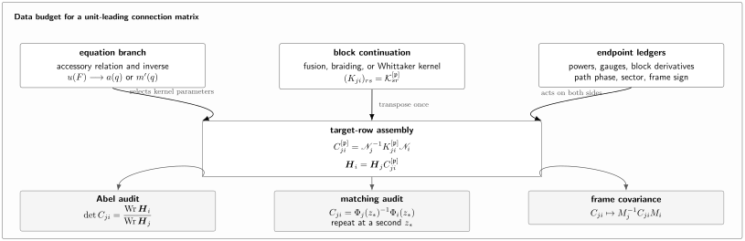
The accessory inverse selects the internal branch used by the exact kernel, while the two endpoint ledgers supply powers, gauges, derivative dressings, phases, and frame signs. Abel’s determinant is a necessary audit; matching all four entries at ordinary points completes the check.

A vanishing shift leaves a finite derivative

The derivative dressings are sometimes described as “subleading,” but they are order one in the normalized probe. Let $\lambda=b\alpha_{\rm L}$ be any scaled heavy momentum. Fusion with a light $(2,1)$ degenerate field shifts it by

$$\lambda_\theta = \lambda-\frac{\theta b^2}{2}, \qquad \theta=\pm1.$$

Assume a differentiable even-power expansion of the relevant background block,

$$\begin{aligned} \Log\mathfrak F_{\mathrm{bg}}(\lambda;b) ={}& \frac{ f_{\mathrm{cl}}(\lambda) }{b^2} + g_{\mathrm{bg}}(\lambda) \\ &+ b^2h_{\mathrm{bg}}(\lambda) + O(b^4). \end{aligned}$$

Taylor expansion before taking the limit gives

$$\begin{aligned} \Log \frac{ \mathfrak F_{\mathrm{bg}}(\lambda_\theta;b) }{ \mathfrak F_{\mathrm{bg}}(\lambda;b) } ={}& -\frac{\theta}{2} \partial_\lambda f_{\mathrm{cl}} \\ &+ b^2 \left[ \frac18 \partial_\lambda^2f_{\mathrm{cl}} - \frac{\theta}{2} \partial_\lambda g_{\mathrm{bg}} \right] \\ &+ O(b^4). \end{aligned}$$

Consequently,

$$\lim_{b\to0} \frac{ \mathfrak F_{\mathrm{bg}}(\lambda_\theta;b) }{ \mathfrak F_{\mathrm{bg}}(\lambda;b) } = \exp \left[ -\frac{\theta}{2} \partial_\lambda f_{\mathrm{cl}} \right].$$

The shift vanishes, but it acts on an exponent of order $b^{-2}$. This is the origin of factors such as

$$e^{-sF_0/2}, \qquad e^{-sF_1/2}, \qquad e^{-\sigma F_a/2}, \qquad e^{-rF_m/2}.$$

They are finite normalization data, not changes in the leading local exponents.

Three derivatives have different jobs:

Derivative	Role
$\partial_t f$ or $L\partial_LF$	Fixes the oper accessory
$\partial_{a_i}F$	Normalizes a degenerate branch at endpoint $i$
$\partial_aF$, $\partial_mF$, or $\partial_{m'}F_D$	Normalizes an intermediate or irregular channel

The modulus derivative and the momentum derivatives cannot be exchanged. They differentiate different data while holding different variables fixed.

Symmetric ratios isolate the next order

Put

$$R_\theta(b) := \frac{ \mathfrak F_{\mathrm{bg}}(\lambda_\theta;b) }{ \mathfrak F_{\mathrm{bg}}(\lambda;b) }.$$

The two sign combinations obey

$$\begin{aligned} \Log R_+ - \Log R_- ={}& -\partial_\lambda f_{\mathrm{cl}} - b^2\partial_\lambda g_{\mathrm{bg}} + O(b^4), \\ \Log R_+ + \Log R_- ={}& \frac{b^2}{4} \partial_\lambda^2f_{\mathrm{cl}} + O(b^4). \end{aligned}$$

These formulas give a clean finite-$b$ diagnostic. After subtracting the leading derivative, the residual should scale by a factor of four under $b\mapsto b/2$. The antisymmetric residual measures $\partial_\lambda g_{\mathrm{bg}}$; the symmetric residual measures the Hessian of the classical action.

Leading and subleading orders

For a generic, nonzero entry of a unit-leading classical ODE matrix, $g_{\mathrm{bg}}$ does not contribute at order $b^0$ to the shifted ratio above. Its difference begins at order $b^2$. The leading matrix therefore needs:

• the complete classical action in the chosen normalization;
• its relevant modulus and momentum derivatives;
• the leading classical limit of the exact degenerate kernel;
• exact local-coordinate, gauge, path, and sector data.

To compute the first $b^2$ correction, one must add all contributions at that order, not only one convenient term:

$$\begin{aligned} \text{first correction} = {}& \text{Hessian of }f_{\mathrm{cl}} \\ &+ \partial g_{\mathrm{bg}} + \text{finite-}b\text{ kernel correction} \\ &+ \text{corrected probe and gauge normalization}. \end{aligned}$$

Absolute chiral or physical coefficients can contain order-one three-point, reflection, pairing, or flux factors even when $g_{\mathrm{bg}}$ cancels from the unit-leading ODE ratio. A saddle evaluation of an integral fusion transform can also contribute a Hessian determinant. Such quantities belong to the declared chiral or physical observable, not automatically to the unit-leading scalar ODE matrix.

If a leading entry vanishes, two exponents coalesce, or a generic Verma-module inverse develops a pole, the power counting can change and subleading terms may become decisive. Page 7 treats those singular limits rather than substituting them into the generic formulas here.

A regular target is one diagonal conversion on each side

The general-Heun endpoint assembly is the regular-singular prototype. In its notation,

$$\boldsymbol H_0 = \boldsymbol H_tC_{t0}, \qquad C_{t0} = \mathscr N_t^{-1} M_{\mathrm{fr}} \mathscr N_0.$$

Here $(M_{\mathrm{fr}})_{rs}=\mathcal M_{sr}$ is the transpose of the source-first degenerate fusion array. The matrices $\mathscr N_0,\mathscr N_t$ contain local powers, scalar-gauge constants, and the external derivatives of the classical block. Expanding this product gives all four gamma-function entries in the general-Heun fusion core.

This compact form also says what the gamma kernel cannot know. It does not know which Frobenius coordinate was assigned leading coefficient one, which logarithm defines a fractional power, or which $t$-independent normalization was added to the classical block. Those choices enter only through the two $\mathscr N$ matrices.

Confluent-Heun endpoint matrices

The sectorial case makes the normalization budget more visible. Use the standard confluent-Heun equation

$$y'' + \left( \frac{\gamma}{z} + \frac{\delta}{z-1} + L \right)y' + \frac{\alpha z-q}{z(z-1)}y =0$$

and the common normal-form gauge

$$P(z) = e^{-Lz/2} z^{-\gamma/2} (1-z)^{-\delta/2}.$$

Put

$$a_0=\frac{1-\gamma}{2}, \qquad a_1=\frac{1-\delta}{2},$$

and keep the full accessory dictionary, logarithms, and frame definitions of the confluent-Heun gauge ledger. The ordered regular frames are

$$\boldsymbol H_0 = \left( H_{0,-},H_{0,+} \right), \qquad \boldsymbol H_1 = \left( H_{1,-},H_{1,+} \right),$$

while the sectorial infinity frame is

$$\boldsymbol Y_\infty^{(\eta)} = \left( Y_+^{(\eta)},Y_-^{(\eta)} \right).$$

For a lateral ray on which

$$\arg(1-z)=-\eta\pi, \qquad \eta=\pm1,$$

write

$$\chi_\eta := e^{\eta\ii\pi\delta/2}.$$

The square $\chi_\eta^2$ is the phase that enters the Wronskian ratio.

The sign and chart conventions used in the remaining formulas are:

Symbol	Meaning and order
$\boldsymbol H_0,\boldsymbol H_1$	Regular frames ordered $(-,+)$
$\boldsymbol Y_\infty$	Infinity frame ordered $(+,-)$
$s$ in a source-first array	Source sign
$r$ in a source-first array	Target sign
$K_{ji}$	Target-row matrix: target index first, source index second
$\eta$	Choice of the two displayed lateral determinations
$k$	General sector index under repeated continuation
$m$	Fixed irregular/background momentum
$m'$	Internal coordinate of the dual large-$L$ chart
$\mu,\rho$	Abbreviations $m'-m$ and $2m'-m$

Every block derivative is taken at fixed remaining arguments and fixed logarithms before the accessory inverse is substituted. With

$$\mathcal A(z) := e^{-Lz} z^{-\gamma} (1-z)^{-\delta},$$

the three declared unit-leading frames satisfy

$$\begin{aligned} \operatorname{Wr} \left[ H_{0,-},H_{0,+} \right] &= 2a_0\mathcal A(z), \\ \operatorname{Wr} \left[ H_{1,-},H_{1,+} \right] &= -2a_1e^L\mathcal A(z), \\ \operatorname{Wr} \left[ Y_+^{(\eta)},Y_-^{(\eta)} \right] &= -L\chi_\eta^{-2}\mathcal A(z). \end{aligned}$$

These exact Abel normalizations are the target that both asymptotic block charts must reproduce.

Small-parameter chart

The block entries in this subsection are all-orders formal small-$L$ identities, conditional on the derivative-compatible semiclassical block limit stated on the preceding page’s scope statement. The unit-leading endpoint conversions and the Abel Wronskian laws are exact for the declared ODE frames.

Let

$$F_\nu:=\partial_\nu F, \qquad \nu\in \left\{ a_0,a_1,a,m \right\},$$

with the abbreviations $F_0,F_1,F_a,F_m$ used below. The block-to-ODE conversions forced by the unit-leading local terms are

$$\begin{aligned} \boldsymbol H_0 &= P\boldsymbol B_0 \mathscr N_0, \\ \boldsymbol H_1 &= P\boldsymbol B_1 \mathscr N_1, \\ \boldsymbol Y_\infty^{(\eta)} &= P\boldsymbol D_\infty^{(\eta)} \mathscr N_\infty^{(\eta)}, \end{aligned}$$

where

$$\mathscr N_0 = \begin{pmatrix} e^{-F_0/2}&0\\ 0&e^{F_0/2} \end{pmatrix},$$ $$\mathscr N_1 = e^{L/2} \begin{pmatrix} e^{-F_1/2}&0\\ 0&e^{F_1/2} \end{pmatrix},$$

and, in the target order $(+,-)$,

$$\begin{aligned} \mathscr N_\infty^{(\eta)} ={}& \chi_\eta^{-1} \\ &\times \begin{pmatrix} e^{F_m/2}L^{1/2+m}&0\\ 0&e^{-F_m/2}L^{1/2-m} \end{pmatrix}. \end{aligned}$$

All powers use the same selected $\Log L$. The common factor $e^{L/2}$ in $\mathscr N_1$ is the inverse of the gauge value $e^{-L/2}$ at $z=1$. It is not generated by a conformal block and cannot be inferred from the fusion kernel.

Regular to regular

Let

$$\left( M_{\mathrm{fr}} \right)_{rs} = \mathcal M_{sr}(a_0,a_1;a), \qquad s,r=-,+,$$

with $\mathcal M$ defined in the first-kind block connection. Within the formal small-$L$ chart, the complete matrix is

$$\boxed{ C_{10}^{\mathrm{small}} = \mathscr N_1^{-1} M_{\mathrm{fr}} \mathscr N_0. }$$

Equivalently, entrywise,

$$\left( C_{10}^{\mathrm{small}} \right)_{rs} = e^{-L/2} \exp \left[ \frac{ sF_0-rF_1 }{2} \right] \mathcal M_{sr}(a_0,a_1;a).$$

The signs $s,r$ are read as the numbers $-1,+1$. The accessory equation is inverted for $a=a(q)$ before the entries are evaluated, but after the partial derivatives have been taken.

Gamma reflection gives

$$\det M_{\mathrm{fr}} = -\frac{a_0}{a_1}.$$

Since

$$\det\mathscr N_0=1, \qquad \det\mathscr N_1=e^L,$$

the exact Abel determinant of the declared ODE frames is

$$\det C_{10}^{\mathrm{small}} = -\frac{a_0}{a_1}e^{-L}.$$

Abel’s identity gives the same result from the unit-leading zero- and one-frames. In particular, the missing factor $e^{-L/2}$ in each entry would produce a determinant error by $e^L$.

Why the endpoint factor is written explicitly

The block-to-standard-function identification printed in Bonelli et al., §4.2, appears to omit the common $e^{L/2}$ at $z=1$. The local gauge and the Abel determinant both require it. The formulas here are assembled from the declared unit-leading germs; this is an apparent normalization inconsistency in the printed display, not a claim of an official erratum.

Regular to sectorial infinity

To keep the target-row convention unambiguous, denote the source-first collision array in the small-$L$ overlap factorization by $\mathcal K_{\mathrm{raw}}^{\mathrm{sf},(\eta)}$. It is

$$\begin{aligned} \left( \mathcal K_{\mathrm{raw}}^{\mathrm{sf},(\eta)} \right)_{sr} ={}& \sum_{\sigma=\pm} \mathcal M_{s\sigma}(a_1,a;a_0) \mathcal N_{-\sigma,r}^{(\eta)}(a,m) \\ &\times L^{\sigma a} e^{-\sigma F_a/2}. \end{aligned}$$

Its identification with the declared second-kind frame requires

$$\mathcal K^{\mathrm{sf},(\eta)} = \mathcal K_{\mathrm{raw}}^{\mathrm{sf},(\eta)}J_\infty, \qquad J_\infty = \operatorname{diag}(1,-1).$$

Equivalently, set

$$j_+=1, \qquad j_-=-1,$$

so that

$$\mathcal K_{sr}^{\mathrm{sf},(\eta)} = j_r \left( \mathcal K_{\mathrm{raw}}^{\mathrm{sf},(\eta)} \right)_{sr}.$$

The corresponding target-row matrix is

$$K_{\infty1}^{(\eta)} := \left( \mathcal K^{\mathrm{sf},(\eta)} \right)^{\mathsf T}.$$

With

$$\boldsymbol H_1 = \boldsymbol Y_\infty^{(\eta)} C_{\infty1}^{(\eta)},$$

the normalized matrix is

$$\boxed{ C_{\infty1}^{(\eta)} = \left( \mathscr N_\infty^{(\eta)} \right)^{-1} K_{\infty1}^{(\eta)} \mathscr N_1. }$$

Its individual target-row entries are

$$\begin{aligned} \left( C_{\infty1}^{(\eta)} \right)_{rs} ={}& \chi_\eta e^{L/2} j_r L^{-1/2-rm} \\ &\times \exp \left[ \frac{ sF_1-rF_m }{2} \right] \\ &\times \sum_{\sigma=\pm} \mathcal M_{s\sigma}(a_1,a;a_0) \mathcal N_{-\sigma,r}^{(\eta)}(a,m) \\ &\hspace{6em}\times L^{\sigma a} e^{-\sigma F_a/2}. \end{aligned}$$

The formula has four logically distinct layers: the $\mathcal M \mathcal N$ kernel, the internal-channel dressing, the source normalization, and the sectorial target normalization. The sign $j_r$ belongs to the last identification; it does not alter the exact Whittaker identity defining $\mathcal N$.

The source-first and target-row matrices have the same determinant:

$$\det\mathcal K^{\mathrm{sf},(\eta)} = \det K_{\infty1}^{(\eta)} = 2a_1.$$

Moreover,

$$\det\mathscr N_1=e^L, \qquad \det\mathscr N_\infty^{(\eta)} = \chi_\eta^{-2}L.$$

Therefore the formal block matrix reproduces the exact Abel determinant

$$\det C_{\infty1}^{(\eta)} = \frac{ 2a_1 }{L} e^L \chi_\eta^2.$$

The entrywise block representation is an all-orders formal small-$L$ identity. The determinant statement is exact for the declared ODE frames and is reproduced directly by their Abel Wronskians. Without $J_\infty$, the sign would be wrong; without $e^{L/2}$, the exponential factor would be wrong.

Composition supplies a third audit:

$$C_{\infty0}^{(\eta)} = C_{\infty1}^{(\eta)} C_{10}^{\mathrm{small}}, \qquad \det C_{\infty0}^{(\eta)} = -\frac{2a_0}{L}\chi_\eta^2.$$

The factors $e^{\pm L}$ cancel because the source has moved from $z=1$ to $z=0$.

Large-parameter chart

The block entries in this subsection are formal large-$L$ asymptotic identities under the corresponding dual-block exponentiation hypothesis. The endpoint conversions follow exactly from the stated leading terms, and the Abel determinant laws of the actual ODE frames remain exact. No equality of resummed small- and large-$L$ charts is assumed.

The large-$L$ chart uses a different internal coordinate $m'$ and the dual block $F_D$. Write

$$F_{D,0} = \partial_{a_0}F_D, \quad F_{D,1} = \partial_{a_1}F_D, \quad F_{D,m} = \partial_mF_D, \quad F_{D,m'} = \partial_{m'}F_D.$$

For compact formulas also set

$$\mu:=m'-m, \qquad \rho:=2m'-m.$$

The unit-leading conversions now contain powers absent from the small-$L$ chart:

$$\mathscr N_0^{D} = \begin{pmatrix} L^{a_0}e^{-F_{D,0}/2}&0\\ 0&L^{-a_0}e^{F_{D,0}/2} \end{pmatrix},$$ $$\mathscr N_1^{D} = e^{L/2} \begin{pmatrix} L^{a_1}e^{-F_{D,1}/2}&0\\ 0&L^{-a_1}e^{F_{D,1}/2} \end{pmatrix},$$

and

$$\begin{aligned} \mathscr N_\infty^{D,(\eta)} ={}& \chi_\eta^{-1} \\ &\times \begin{pmatrix} e^{L/2} e^{F_{D,m}/2} L^{1/2-(m'-m)} &0 \\ 0& e^{-L/2} e^{-F_{D,m}/2} L^{1/2+(m'-m)} \end{pmatrix}. \end{aligned}$$

These matrices follow from the displayed one-end and infinity asymptotics in the large-$L$ block chart, together with the zero-end analogue obtained by endpoint exchange. They also show why replacing $F$ by $F_D$ in a small-$L$ component formula is insufficient: the powers of $L$ and the endpoint exponentials change at the same time.

Regular to regular in the dual chart

Define the source-first block kernel

$$\begin{aligned} \left( \mathcal Q^{D,\mathrm{sf}} \right)_{sr} ={}& \sum_{\sigma=\pm} \frac{ \Gamma(1+2s a_0) \Gamma(-2r a_1) }{ \Gamma\left( \frac12+s a_0-\sigma m' \right) \Gamma\left( \frac12-r a_1-\sigma\mu \right) } \\ &\times e^{\sigma L/2} L^{-\sigma\rho} e^{-\sigma F_{D,m'}/2} \\ &\times \exp \left[ \frac{\ii\pi}{2} (1-\sigma) \left( s a_0-r a_1-\rho \right) \right]. \end{aligned}$$

This is the expanded product of a Whittaker kernel and an inverse Whittaker kernel. Writing it explicitly removes any ambiguity about the row order of that inverse. The displayed phase uses the same clockwise Whittaker branch and continuation homotopy, which we denote $[\mathfrak p_+]$; $C_{10}^{D}$ is shorthand for $C_{10}^{D,[\mathfrak p_+]}$. Other homotopy classes require the corresponding monodromy transport. Define the target-row transpose by

$$K_{10}^{D} := \left( \mathcal Q^{D,\mathrm{sf}} \right)^{\mathsf T}.$$

The normalized matrix is

$$C_{10}^{D} = \left( \mathscr N_1^{D} \right)^{-1} K_{10}^{D} \mathscr N_0^{D},$$

or, entrywise,

$$\boxed{ \left( C_{10}^{D} \right)_{rs} = e^{-L/2} L^{-s a_0+r a_1} \exp \left[ \frac{ sF_{D,0}-rF_{D,1} }{2} \right] \left( \mathcal Q^{D,\mathrm{sf}} \right)_{sr}. }$$

The exact kernel identity gives

$$\det\mathcal Q^{D,\mathrm{sf}} = \det K_{10}^{D} = -\frac{a_0}{a_1}.$$

Therefore the large-$L$ formal matrix obeys the same ODE determinant law as the small-$L$ matrix:

$$\det C_{10}^{D} = -\frac{a_0}{a_1}e^{-L}.$$

Agreement of the determinant does not identify the two asymptotic series entry by entry. It only confirms that both charts use the same unit-leading ODE frames.

Regular to infinity in one reference sector

The printed large-$L$ block relation fixes the clockwise Whittaker determination

$$\Log\!\left(e^{-\ii\pi}x\right) = \Log x-\ii\pi.$$

In the convention used here this is the reference lateral ray $\arg(1-z)=-\pi$, hence $\eta=+1$. Its rigid source-first kernel is

$$\left( \mathcal K_{\infty1}^{D,\mathrm{sf},(+)} \right)_{sr} = \mathcal N_{s,-r}^{(+)} \left( a_1,\mu \right).$$

Explicitly,

$$\begin{aligned} \mathcal N_{s,-r}^{(+)}(a_1,\mu) ={}& \frac{ \Gamma(1+2s a_1) }{ \Gamma\left( \frac12+s a_1+r\mu \right) } \\ &\times \exp \left[ \frac{\ii\pi}{2} (1+r) \left( \frac12-\mu+s a_1 \right) \right]. \end{aligned}$$

Define the target-row matrix

$$K_{\infty1}^{D,(+)} := \left( \mathcal K_{\infty1}^{D,\mathrm{sf},(+)} \right)^{\mathsf T}.$$

Consequently,

$$C_{\infty1}^{D,(+)} = \left( \mathscr N_\infty^{D,(+)} \right)^{-1} K_{\infty1}^{D,(+)} \mathscr N_1^D,$$

with entries

$$\boxed{ \begin{aligned} \left( C_{\infty1}^{D,(+)} \right)_{rs} ={}& \chi_+ e^{(1-r)L/2} L^{-1/2-s a_1+r\mu} \\ &\times \exp \left[ \frac{ sF_{D,1}-rF_{D,m} }{2} \right] \\ &\times \mathcal N_{s,-r}^{(+)} \left( a_1,\mu \right). \end{aligned} }$$

Here no $J_\infty$ is inserted:

$$\det \left[ \mathcal N_{s,-r}^{(+)} \right] = 2a_1$$

in the stated row and column orders. Adding the small-$L$ collision-frame sign to this independently normalized large-$L$ kernel would violate the Wronskian determinant. In the reference sector the result is

$$\det C_{\infty1}^{D,(+)} = \frac{ 2a_1 }{L} e^L \chi_+^2.$$

The opposite lateral matrix is not obtained by replacing $\chi_+$ with $\chi_-$ in the displayed entries. The scalar phase $\chi_\eta$ records only the gauge branch; the sectorial jump belongs to a different kernel $\mathcal N^{(\eta)}$, equivalently to Stokes transport. Once that kernel is continued consistently, the pathwise exact Abel law is

$$\det C_{\infty1}^{D,(\eta)} = \frac{2a_1}{L} e^L\chi_\eta^2.$$

The next section gives the matrix transport law that constructs the adjacent sector.

Re-derive the large-parameter translations

Several component translations printed in Bonelli et al., §4.2, appear to omit the endpoint factors $e^{L/2}$ and $L^{-s a_i}$; nearby lines also contain inconsistent infinity sign labels and powers. The compact block kernels remain useful, but the standard-function matrix should be rebuilt from the local block asymptotics as above. The determinant provides an immediate independent check.

A comparison ledger for the printed translations

Readers checking the formulas against the source can use the following diagnostic ledger. Each row is an apparent transcription or normalization inconsistency, not an official erratum.

Printed feature	Unit-leading reconstruction	Audit
Small-$L$ one-end conversion lacks a common endpoint factor	Restore $e^{L/2}$	$\det C_{10}$
Infinity series is displayed with argument $z$ in a connection formula	Use its defining inverse-power argument $z^{-1}$	Large-$z$ series
Small-$L$ collision frame has the opposite relative orientation	Apply $J_\infty$ only in that collision identification	$\det C_{\infty1}$
A small-$L$ infinity component has an inconsistent $F_m$ sign or lateral phase	Derive $-rF_m/2$ and the phase from $\mathscr N_\infty^{-1}K^{\mathsf T}$	Exact Whittaker slice
Large-$L$ finite-end conversions omit powers	Restore $L^{-s a_0}$ and $L^{-s a_1}$	Local leading coefficients
Large-$L$ exponential infinity branch repeats the $+$ sign label	Use the $r=-$ branch	Formal exponential
A component expression places a factor $e^{\mp L/2}$ inside a power of $L$	Keep exponentials and powers separate	Dimensions and Abel determinant
A large-$L$ exponential coefficient uses the opposite sign of $m'$ in one gamma denominator	Use the sign fixed by $\mathcal N_{s,-r}^{(+)}(a_1,\mu)$	Whittaker-kernel definition

The safe procedure is structural: start with a block relation whose sign indices are explicit, derive both $\mathscr N$ matrices from the local leading terms, and multiply them in the frame equation. Copying four expanded components independently discards precisely the redundancy that makes the result auditable.

Adjacent sectors change the target matrix

Suppose the sectorial infinity frames satisfy the book’s right-action law

$$\boldsymbol Y_\infty^{(k+1)} = \boldsymbol Y_\infty^{(k)}S_k.$$

For one fixed regular source frame,

$$\boldsymbol H_i = \boldsymbol Y_\infty^{(k)} C_{\infty i}^{(k)} = \boldsymbol Y_\infty^{(k+1)} C_{\infty i}^{(k+1)}.$$

Therefore

$$C_{\infty i}^{(k+1)} = S_k^{-1} C_{\infty i}^{(k)}.$$

The block-to-one-sector kernel and the Stokes matrix have different jobs. The former constructs $C_{\infty i}^{(k)}$; the latter changes its target frame. Folding $S_k$ into an unlabeled “irregular connection coefficient” destroys the information needed to continue it. The phase $\chi_\eta$ tracks only the scalar-gauge branch, so changing $\chi_\eta$ alone cannot implement this matrix jump. In particular, when $\delta=0$ the two phases coincide even though $S_k$ can be nontrivial. On a fixed analytic branch $\det S_k=1$, as required by the unchanged Abel determinant.

A factor ablation catches what a determinant cannot

The genuinely four-singular general-Heun slice provides an entrywise test of the assembly theorem. A direct Frobenius match at $z=t/2$ is compared with the level-two classical-block matrix: $q_{\mathrm H}$ and both endpoint derivatives are truncated consistently through $t^2$. The same calculation is then repeated after setting both endpoint derivatives to zero while retaining the fusion kernel and all coordinate powers.

$t$	Fully dressed level-two matrix	Endpoint derivatives omitted
$0.08$	$9.12\times10^{-5}$	$1.40\times10^{-2}$
$0.04$	$1.09\times10^{-5}$	$6.83\times10^{-3}$
$0.02$	$1.33\times10^{-6}$	$3.37\times10^{-3}$
$0.01$	$1.64\times10^{-7}$	$1.68\times10^{-3}$

The fully dressed error decreases by approximately eight when $t$ is halved, as expected from the omitted $O(t^3)$ terms. The ablated error decreases only by approximately two because the missing derivative normalization starts at $O(t)$.

At $t=0.04$, all three computed determinants agree to the 18 digits reported here:

$$\det C_{\mathrm{direct}} \approx \det C_{\mathrm{block}} \approx \det C_{\mathrm{ablated}} \approx -1.03319670758600654.$$

The block and ablated determinants obey the Abel value algebraically; the direct-series determinant is numerical. The derivative factors have reciprocal determinant and cancel from the Abel law. This example makes the hierarchy of tests explicit:

1. a determinant failure proves the matrix is wrong;
2. a determinant success does not prove its entries are right;
3. matching at two ordinary points tests the entire matrix.

The general-Heun reproducibility script generates the table and the ablation. For one row, run:

python3 public/code/advanced-ode/general-heun-connection-check.py \
  --t 0.04 --order 2 --terms 120 --dps 50 \
  --no-table --show-ablation --check-second-point

The reported run used Python 3.10.16, mpmath 1.3.0, 120 Frobenius terms, 50 decimal digits, and positive-real branches with $0<t<2/3$; its measured wall time was $0.06$ seconds on the audit machine. At $t=0.04$, changing the series length from 80 through 180 terms leaves the displayed digits stable. Repeating the direct match at $z=t/3$ changes the matrix by only $2.28\times10^{-22}$ relative to the $z=t/2$ result. The script rejects under-resolved precision or series-length inputs and warns when the direct-series determinant signals poor convergence near a disk boundary.

The exact Whittaker benchmark on the preceding page’s exact benchmark independently checks a sectorial kernel, its derivatives, Wronskian determinant, and adjacent-sector matrix law.

A reusable assembly workflow

For a new conformal-block connection problem:

1. Fix the scalar equation. State its gauge, parameters, and the exact accessory coordinate used by the block.
2. Declare both ODE frames. Give their order, local coordinate, unit-leading behavior, logarithms, and continuation path.
3. Choose one block chart. Do not mix $F$ with $F_D$, or a $c_{\mathrm{Vir}}=1$ Fourier block with a classical block.
4. Invert the accessory relation. Select $a(q)$ or $m'(q)$ and verify the relevant inverse Jacobian is nonzero.
5. Differentiate before substitution. Hold the other block data fixed while computing the external and internal derivatives.
6. Build the target-row kernel. Transpose a source-first coefficient array exactly once.
7. Derive the endpoint ledgers. Read every factor in $\mathscr N_i,\mathscr N_j$ from a declared local or asymptotic leading term.
8. Multiply the three factors. Use $C_{ji}=\mathscr N_j^{-1}K_{ji}\mathscr N_i$ before expanding components.
9. Audit independently. Check the Abel determinant, match at two ordinary points, and verify any sector-change law.
10. Add physical normalization last. Only then contract with boundary vectors or include reflection, pairing, flux, or vertex factors.

Record the claimed accuracy together with the result. “Leading classical,” “through $L^N$,” “through $L^{-N}$,” and “including the first $b^2$ correction” are different deliverables.

Common pitfalls

Calling the fusion kernel the connection matrix. The kernel acts on block representatives. The two endpoint conversions are required before its entries refer to unit-leading ODE functions.

Using the accessory derivative as an endpoint derivative. $\partial_t f$ selects the equation, while $\partial_{a_i}f$ fixes a probe normalization. They are partial derivatives with different held data.

Differentiating after solving for the internal lift. The shifted block holds the internal channel fixed. Applying the chain rule to $F(a(q),\ldots)$ inserts a term not present in the fusion limit.

Evaluating the gauge at infinity. An irregular target is normalized by an asymptotic comparison in a sector. There is no finite endpoint value $P(\infty)$.

Carrying a collision-frame sign into every chart. The small-$L$ kernel needs $J_\infty$ for the declared frame; the large-$L$ kernel already has the correct column orientation. The Wronskian decides.

Assuming the order-one block term always contributes. $g_{\mathrm{bg}}$ cancels from a generic leading shifted ratio, but it enters the first $b^2$ correction and can survive in absolute chiral or physical normalizations.

Calling an ODE entry a physical amplitude. A unit-leading connection entry changes under endpoint rescaling. A physical observable must include the associated boundary or flux conventions.

Exercises

1. Catch a source-first transpose error

A continuation formula is printed source first:

$$\mathcal B_{i,s} = \sum_{r=1}^2 \mathcal A_{sr}\mathcal B_{j,r}, \qquad \mathcal A = \begin{pmatrix} a&b\\ c&d \end{pmatrix}.$$

Let

$$\mathscr N_i=\operatorname{diag}(p,q), \qquad \mathscr N_j=\operatorname{diag}(u,v).$$

Construct the target-row connection matrix $C_{ji}$. Which coefficient multiplies $H_{j,2}$ in the expansion of $H_{i,1}$? Show why a determinant test alone cannot detect the error made by omitting the transpose.

Solution

The first index of $\mathcal A_{sr}$ labels a source solution, whereas the row of a frame matrix labels a target solution. Thus

$$K_{ji} = \mathcal A^{\mathsf T} = \begin{pmatrix} a&c\\ b&d \end{pmatrix}.$$

The two-sided conversion gives

$$C_{ji} = \mathscr N_j^{-1} K_{ji}\mathscr N_i.$$

Hence

$$\begin{aligned} C_{ji} &= \begin{pmatrix} u^{-1}&0\\ 0&v^{-1} \end{pmatrix} \begin{pmatrix} a&c\\ b&d \end{pmatrix} \begin{pmatrix} p&0\\ 0&q \end{pmatrix} \\ &= \begin{pmatrix} ap/u&cq/u\\ bp/v&dq/v \end{pmatrix}. \end{aligned}$$

The first column expands $H_{i,1}$, so the requested coefficient is $bp/v$. Omitting the transpose would instead give $cp/v$. Yet

$$\det\!\left( \mathscr N_j^{-1}\mathcal A^{\mathsf T}\mathscr N_i \right) = \det\!\left( \mathscr N_j^{-1}\mathcal A\mathscr N_i \right),$$

because $\det\mathcal A^{\mathsf T}=\det\mathcal A$. Direct entrywise matching, not the Abel determinant alone, catches this transpose error.

2. Recover the first correction to a shifted block

Let

$$\lambda_\theta = \lambda-\frac{\theta b^2}{2},$$

and use the expansion of $\Log\mathfrak F_{\mathrm{bg}}$ on this page. Find $\Log R_\theta$ through order $b^2$.

Solution

Taylor expansion gives

$$\begin{aligned} f(\lambda_\theta)-f(\lambda) ={}& -\frac{\theta b^2}{2}f' + \frac{b^4}{8}f'' + O(b^6), \\ g(\lambda_\theta)-g(\lambda) ={}& -\frac{\theta b^2}{2}g' + O(b^4). \end{aligned}$$

After dividing the first line by $b^2$,

$$\Log R_\theta = -\frac{\theta}{2}f' + b^2 \left( \frac18f'' - \frac{\theta}{2}g' \right) + O(b^4).$$

The $b^2h$ term changes only at order $b^4$.

3. Recover both confluent-Heun determinant laws

Use the determinants of the three small-$L$ endpoint matrices and the kernel identities

$$\det M_{\mathrm{fr}} = -\frac{a_0}{a_1}, \qquad \det K=2a_1.$$

Find $\det C_{10}$ and $\det C_{\infty1}^{(\eta)}$.

Solution

For the two finite endpoints,

$$\det\mathscr N_0=1, \qquad \det\mathscr N_1=e^L.$$

Therefore

$$\det C_{10} = \frac1{e^L} \left( -\frac{a_0}{a_1} \right) = -\frac{a_0}{a_1}e^{-L}.$$

At infinity,

$$\det\mathscr N_\infty^{(\eta)} = \chi_\eta^{-2}L.$$

Hence

$$\det C_{\infty1}^{(\eta)} = \frac{ e^L }{ \chi_\eta^{-2}L } (2a_1) = \frac{2a_1}{L} e^L\chi_\eta^2.$$

4. Propagate an adjacent-sector change

Given

$$\boldsymbol Y_\infty^{(k+1)} = \boldsymbol Y_\infty^{(k)}S_k,$$

derive the relation between $C_{\infty i}^{(k+1)}$ and $C_{\infty i}^{(k)}$.

Solution

Write the same source frame in the two target frames:

$$\boldsymbol H_i = \boldsymbol Y_\infty^{(k)} C_{\infty i}^{(k)} = \boldsymbol Y_\infty^{(k)} S_kC_{\infty i}^{(k+1)}.$$

Linear independence gives

$$C_{\infty i}^{(k)} = S_kC_{\infty i}^{(k+1)},$$

and therefore

$$C_{\infty i}^{(k+1)} = S_k^{-1}C_{\infty i}^{(k)}.$$

5. Show that a boundary scalar is frame independent

Let a scalar boundary function be

$$\mathcal Q = \ell_j^{\mathsf T} C_{ji}v_i.$$

If the endpoint frames change by $M_i,M_j$, find the transformations of $v_i$ and $\ell_j$ that leave $\mathcal Q$ unchanged.

Solution

The connection matrix changes to

$$\widetilde C_{ji} = M_j^{-1}C_{ji}M_i.$$

Choose

$$\widetilde v_i = M_i^{-1}v_i, \qquad \widetilde\ell_j^{\mathsf T} = \ell_j^{\mathsf T}M_j.$$

Then

$$\begin{aligned} \widetilde{\mathcal Q} &= \ell_j^{\mathsf T}M_j M_j^{-1}C_{ji}M_i M_i^{-1}v_i \\ &= \ell_j^{\mathsf T}C_{ji}v_i = \mathcal Q. \end{aligned}$$

The scalar can be invariant even though every matrix entry changes.

6. Explain the ablation paradox

Why does deleting the endpoint derivative factors in the general-Heun test leave the determinant unchanged while spoiling the entries?

Solution

The derivative dressings are diagonal with reciprocal entries, so each has determinant one. Deleting them therefore leaves

$$\frac{ \det\mathscr N_i }{ \det\mathscr N_j } \det K_{ji}$$

unchanged. Their individual diagonal entries are not one, however, so they rescale different rows and columns and change all four connection coefficients. Abel’s determinant is necessary but not sufficient; direct matching supplies the missing entrywise test.

References

• G. Bonelli, C. Iossa, D. Panea Lichtig, and A. Tanzini, “Irregular Liouville Correlators and Connection Formulae for Heun Functions”, Communications in Mathematical Physics 397 (2023), 635–727. Sections 3.1–3.2 derive the regular and confluent block kernels and their semiclassical limits; Sections 4.1–4.2 translate them to Heun equations. This page reconstructs the unit-leading endpoint factors directly where the printed component translations appear inconsistent.
• M. Beşken, S. Datta, and P. Kraus, “Semi-classical Virasoro Blocks: Proof of Exponentiation”, Journal of High Energy Physics 2020 (1), 109. Proves exponentiation of Virasoro blocks in the simultaneous large-central-charge, heavy-weight limit.
• J. Teschner, “Liouville Theory Revisited”, Classical and Quantum Gravity 18 (2001), R153–R222. Develops chiral operators, braiding, and the distinction between chiral and full Liouville normalizations.
• O. Lisovyy and A. Naidiuk, “Perturbative Connection Formulas for Heun Equations”, Journal of Physics A: Mathematical and Theoretical 55 (2022), 434005. Gives an independent ODE-side large-order construction and comparison for general, confluent, and reduced confluent Heun equations.
• NIST Digital Library of Mathematical Functions, §13.14, “Whittaker Functions”, §31.12, “Confluent Forms of Heun’s Equation”, and §31.18, “Methods of Computation”. These provide the rigid special-function identities, confluent equations, and direct numerical matching framework used in the independent audits.

The next page separates Frobenius resonance from Kac or Zamolodchikov poles. That distinction is essential precisely when the generic endpoint matrices or shifted-block expansion used here cease to be uniform.