Spectral Curves, Turning Points, Poles, and Sheets

The leading equation $P_0^2=R_0$ does not merely ask for a square root of a function. Under a coordinate change, $R_0$ is the coefficient of a quadratic differential. Its square root is therefore a one-form on a generally branched double cover. Once that cover is compactified and normalized, zeros, poles, infinity, and coalescing turning points fit into one local rule:

$$\operatorname{ord}_p(\phi_0)\ \text{is odd} \quad\Longleftrightarrow\quad \pi\ \text{ramifies over }p.$$

This parity test is elementary, but it prevents several common global errors. A double zero is not a branch point after normalization, a simple pole is a branch point even though the lifted WKB one-form is regular there, and infinity can supply the branch point that an affine drawing appears to be missing.

Page question

How does the divisor of the leading quadratic differential determine the sheets, ramification, poles of the WKB one-form, and genus of the spectral cover?

Status ledger

Statement	Status
Coordinate invariance of $\phi_0=R_0\,\dd z^2$	Exact leading-order identity
Odd-order ramification rule	Exact statement about the normalized cover
Riemann–Hurwitz genus count	Exact for a compact, connected normalized cover
Turning-point motion away from the discriminant	Local holomorphic statement
Topology at a discriminant value	Singular degeneration; normalize the special fiber separately
Stokes curves, Borel sums, and connection formulae	Not supplied on this page

The leading potential is a quadratic differential

Take the $\hbar$-dependent normal form

$$\hbar^2\psi'' = R(z,\hbar)\psi, \qquad R(z,\hbar) = R_0(z)+O(\hbar).$$

For an $\hbar$-independent local biholomorphism $z=z(w)$, Page 1 showed that

$$\widetilde R_0(w) = \left( \frac{\dd z}{\dd w} \right)^2 R_0(z(w)).$$

Consequently,

$$\phi_0 := R_0(z)\,\dd z^2$$

is a meromorphic quadratic differential on the base Riemann surface $C$. The function $R_0$ by itself is coordinate dependent; $\phi_0$ is the geometric object.

For the global statements on this page, $C$ is compact and connected and $\phi_0\not\equiv0$ is meromorphic. An affine problem is first equipped with a specified compactification, so its points at infinity are part of the divisor.

Let $D_\infty$ be the pole set of $\phi_0$ and let $K_C$ be the canonical bundle. Over $C^\circ=C\setminus D_\infty$, the unresolved square-root curve lies in the total space of $K_C$:

$$\Sigma_{\mathrm{raw}}^\circ = \left\{ (p,\lambda)\in\operatorname{Tot}(K_C|_{C^\circ}) \ \middle|\ \lambda^{\otimes2}=\phi_0(p) \right\}.$$

Normalize a compactification of this curve over the omitted poles. The resulting WKB spectral cover

$$\pi:\widehat\Sigma\longrightarrow C$$

may be disconnected in the global-square case discussed below. On $\widehat\Sigma$ there is a meromorphic tautological one-form $\lambda_0$ satisfying

$$\lambda_0^{\otimes2} = \pi^*\phi_0.$$

In a coordinate chart,

$$\lambda_0=y\,\dd z, \qquad y^2=R_0(z).$$

Thus the familiar equation $y^2=R_0(z)$ is a local expression, not a license to treat $y$ or $R_0$ as coordinate scalars.

Normalize before reading the geometry

The plane equation $y^2=R_0(z)$ can have nodes, cusps, or reducible components at multiple zeros. Branch points and genus belong to its normalization, not to a sketch of the singular raw curve.

Normalization turns order parity into branching

Let $p\in C$, choose $z(p)=0$, and write

$$\phi_0 = z^m u(z)\,\dd z^2, \qquad u(0)\neq0,$$

where

$$m=\operatorname{ord}_p(\phi_0)\in\mathbb Z.$$

Positive $m$ means a zero, negative $m$ a pole, and $m=0$ an ordinary point. On a small disc, choose a holomorphic square root $q(z)^2=u(z)$.

If $m=2k$ is even, the raw equation factors locally into two branches. Normalization produces two distinct points $p_+$ and $p_-$ above $p$, with

$$\lambda_0 = \pm z^kq(z)\,\dd z.$$

The covering is unramified and

$$\operatorname{ord}_{p_\pm}(\lambda_0) = k = \frac m2.$$

If $m=2k+1$ is odd, introduce the normalized coordinate

$$z=\xi^2.$$

There is one point above $p$, the projection has ramification index $2$, and

$$\begin{aligned} y &= \xi^{\,2k+1}q(\xi^2), \\ \lambda_0 &= 2\xi^{\,2k+2}q(\xi^2)\,\dd\xi. \end{aligned}$$

Hence

$$\operatorname{ord}_{\widehat p}(\lambda_0) = m+1.$$

These formulas remain valid for negative $k$. They prove both the odd-order ramification rule and the lifted order of the WKB one-form. Equivalently, if $e_{\widehat p}\in\{1,2\}$ is the local ramification index, both cases obey

$$2\operatorname{ord}_{\widehat p}(\lambda_0) = e_{\widehat p}m + 2(e_{\widehat p}-1).$$

This follows directly from $\operatorname{ord}_{\widehat p}(\pi^*\dd z) =e_{\widehat p}-1$.

Zeros and poles have different lifts

For zeros, the first two cases are:

Base behavior of $\phi_0$	Covering above the point	Behavior of $\lambda_0$
Simple zero, $m=1$	One ramification point	Zero of order $2$
Double zero, $m=2$	Two unramified points	Simple zero at each point
Zero of odd order $m$	One ramification point	Zero of order $m+1$
Zero of even order $m$	Two unramified points	Zero of order $m/2$ at each point

A simple zero is the ordinary WKB turning point: the two leading Riccati roots coalesce and the recursion of Page 2 becomes singular. A double zero also represents coalesced leading roots, but it is not a branch point after normalization. The singular raw model $y^2=z^2u(z)$ separates into two local sheets.

For poles:

Base behavior of $\phi_0$	Covering above the point	Behavior of $\lambda_0$
Simple pole, $m=-1$	One ramification point	Regular and nonzero
Double pole, $m=-2$	Two unramified points	Simple pole at each point
Odd pole, $m=-(2\ell+1)$, $\ell\geq1$	One ramification point	Pole of order $2\ell$
Even pole, $m=-2\ell$, $\ell\geq1$	Two unramified points	Pole of order $\ell$ at each point

At a double pole, if

$$\phi_0 = \left( \frac{c^2}{z^2}+O(z^{-1}) \right) \dd z^2,$$

then the two lifted one-forms have residues $+c$ and $-c$. Page 5 will keep these residues explicit when periods are regularized.

Terminology at a simple pole is not uniform. This book calls zeros of $\phi_0$ turning points and calls the $m=-1$ case a simple-pole branch point. Modern exact-WKB sources also use “turning point of simple-pole type,” because its local connection problem is turning-point-like. The defining order $m=-1$ is safer than the name.

Sheets are local choices; the involution is global

Away from the odd-order divisor, the cover is locally the disjoint union of two sheets:

$$y=+\sqrt{R_0} \qquad\text{and}\qquad y=-\sqrt{R_0}.$$

The global deck involution

$$\tau:\widehat\Sigma\longrightarrow\widehat\Sigma$$

exchanges them and obeys

$$\tau^*\lambda_0=-\lambda_0.$$

A branch cut is only a device for drawing these local choices in one copy of the base. Crossing a cut changes the displayed sign of $\sqrt{R_0}$; it does not create a singularity of $\widehat\Sigma$. A small loop around an odd-order point lifts to a path that ends on the other sheet. A loop around an even-order point closes on the sheet where it started.

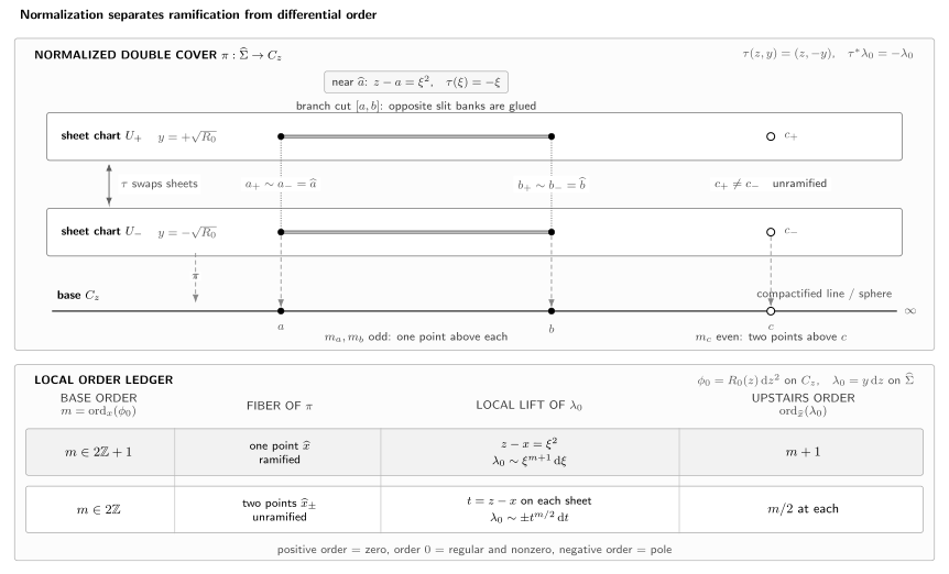
The normalized WKB cover. Odd order of the base quadratic differential produces one ramification point with local coordinate $z=\xi^2$; even order produces two distinct preimages. The tautological one-form $\lambda_0$ is anti-invariant under the deck involution $\tau$.

The same involution organizes all-order WKB geometry. Under the $\hbar$-parity hypothesis of Page 2, the formal phase one-form

$$P_{\mathrm{even}}(z,\hbar)\,\dd z$$

lifts as a single-valued, $\tau$-anti-invariant formal one-form away from its divisor. Its leading term is $\lambda_0$. Higher $R_n$ do not change this leading double cover, although they can add poles to higher WKB coefficients.

Infinity belongs in the divisor

On an affine $z$-plane, introduce

$$\xi=\frac1z.$$

Since $\dd z=-\xi^{-2}\dd\xi$,

$$\phi_0 = R_0(1/\xi)\, \xi^{-4}\dd\xi^2.$$

The factor $\xi^{-4}$ is essential. If $R_0(z)$ is a polynomial of degree $d$, then

$$\operatorname{ord}_\infty(\phi_0) = -(d+4).$$

Thus infinity is a branch point exactly when $d$ is odd. Counting only finite roots would give the wrong parity for the branch divisor and, often, the wrong genus.

The lifted orders are

$$\operatorname{ord}(\lambda_0) = \begin{cases} -d/2-2, & d\ \text{even, at each of two points}, \\ -d-3, & d\ \text{odd, at the ramification point}. \end{cases}$$

Two basic checks are:

$$\begin{array}{c|c|c} R_0(z) & \text{finite odd-order points} & \operatorname{ord}_\infty(\phi_0) \\ \hline z & 0\text{, simple zero} & -5 \\ z^2-a^2,\ a\neq0 & \pm a\text{, simple zeros} & -6 \end{array}$$

The Airy cover branches at $0$ and $\infty$. The Weber cover with $a\neq0$ branches at $\pm a$, while the two points above infinity are unramified.

Riemann–Hurwitz counts handles after normalization

Assume that $C$ is compact of genus $g_C$ and that the normalized double cover is connected. Let $B$ be the number of distinct points of $C$ where $\operatorname{ord}(\phi_0)$ is odd, including poles and points at infinity. Every such point is simply ramified, so Riemann–Hurwitz gives

$$2g_{\widehat\Sigma}-2 = 2(2g_C-2)+B.$$

Equivalently,

$$g_{\widehat\Sigma} = 2g_C-1+\frac B2.$$

In particular, $B$ is even. There is also a divisor check:

$$\sum_{p\in C} \operatorname{ord}_p(\phi_0) = \deg K_C^{\otimes2} = 4g_C-4.$$

The right side is even, so an even number of terms in the sum can be odd. For a polynomial of degree $d\geq1$ with simple roots on $C=\mathbb P^1$,

$$g_{\widehat\Sigma} = \left\lfloor \frac{d-1}{2} \right\rfloor.$$

The hypotheses matter. If

$$\phi_0=\omega^2$$

for a global meromorphic one-form $\omega$, then the normalized cover splits into the two components $\lambda_0=\pm\omega$. The connected genus formula must not be applied to their union. Conversely, a cover with no branch points need not split: its square-root local system can define a connected unramified double cover.

Turning points move until the discriminant vanishes

For the spectral family

$$R_0(z;E)=V(z)-E,$$

a simple turning point $z_t(E)$ satisfies

$$V(z_t(E))=E, \qquad V'(z_t(E))\neq0.$$

The implicit-function theorem gives

$$\frac{\dd z_t}{\dd E} = \frac1{V'(z_t)}.$$

The root moves holomorphically until $V'(z_t)=0$. For a polynomial potential, collisions occur at zeros of

$$\Delta(E) := \operatorname{Disc}_z\!\left(V(z)-E\right).$$

The sign and leading normalization of the discriminant depend on convention; its zero set does not.

For a reduced rational family $R_0=N/D$, the ledger is larger: $\operatorname{Disc}_zN$ detects finite zero collisions, $\operatorname{Disc}_zD$ detects pole collisions, and $\operatorname{Res}_z(N,D)$ detects zero–pole cancellation. Leading-coefficient conditions are still needed for a point moving through infinity.

For a concrete genus-changing family, take

$$V(z)=z^3-3z.$$

Then

$$\Delta(E) = 108-27E^2 = 27(4-E^2).$$

At $E=2$,

$$z^3-3z-2 = (z+1)^2(z-2),$$

and at $E=-2$,

$$z^3-3z+2 = (z-1)^2(z+2).$$

For generic $E$, the three finite simple zeros and the odd-order pole at infinity give $B=4$ and genus $1$. At $E=\pm2$, two simple branch points collide into an even double zero. The normalized special fiber has $B=2$ and genus $0$. The raw curve is singular at the collision, so the special fiber must be normalized before its topology is read.

Locally, if $z_c$ is a nondegenerate critical point of $V$, then

$$\begin{aligned} V(z)-E ={}& \frac12V''(z_c)(z-z_c)^2 \\ &- (E-V(z_c)) + \cdots. \end{aligned}$$

This square-root splitting explains both the divergent derivative $\dd z_t/\dd E$ and the vanishing cycle that Page 4 will place in homology.

Airy and Weber expose the topology

For Airy,

$$y^2=z.$$

The global parameterization

$$z=\xi^2, \qquad y=\xi$$

gives

$$\lambda_0 = y\,\dd z = 2\xi^2\,\dd\xi.$$

The simple turning point becomes a double zero of $\lambda_0$ upstairs, while the order-$5$ pole of $\phi_0$ at infinity becomes an order-$4$ pole of $\lambda_0$. The compactified cover is a sphere.

For Weber with $a\neq0$,

$$y^2=z^2-a^2,$$

the two finite simple zeros are the branch points and infinity has two unramified preimages. Again the cover has genus $0$. In the limit $a\to0$,

$$\phi_0 = z^2\,\dd z^2 = (z\,\dd z)^2.$$

The raw curve becomes nodal and its normalization splits into the two global components $\lambda_0=\pm z\,\dd z$. This is a useful warning: coalescing branch points can change not only the genus but also the connectedness of the normalized special fiber.

What the spectral cover does not determine

The normalized cover determines where the leading momentum changes sheet and supplies the one-form whose periods begin the WKB actions. It does not by itself choose:

• a branch-cut drawing;
• an absolute or relative homology basis;
• a phase of $\hbar$;
• a Stokes graph or summation direction;
• a canonical analytic solution;
• boundary conditions or a quantization rule.

Page 4 adds cycles and intersection pairings. Page 5 defines the regularized all-order periods. Stokes graphs, Borel summation, and analytic connection formulae remain in Chapter 9.

Also keep the cover separate from movable Riccati poles. A zero of a chosen exact solution makes $P_\psi=\hbar\psi'/\psi$ singular, but it does not alter $\phi_0$, its branch divisor, or $\widehat\Sigma$.

Reproducible spectral-cover audit

The spectral-cover check verifies the local order formulas, the contribution from infinity, the Airy and Weber genus counts, the cubic discriminant, and a reducible global-square example. Run

python3 public/code/advanced-ode/wkb-spectral-cover-check.py

The script uses exact SymPy algebra and explicit failures that remain active under optimized Python.

Common pitfalls

Branching at every zero or pole. Ramification is controlled by the parity of the order. A double zero and a double pole are unramified after normalization.

Forgetting that a simple pole is special. It is a ramification point even though $\lambda_0$ is regular and nonzero upstairs. Its exact-WKB connection problem requires separate local analysis.

Counting only finite branch points. The quadratic differential acquires the factor $\xi^{-4}$ at infinity. Omitting it gives an incorrect divisor and genus.

Using the raw plane curve for genus. Multiple roots make the raw curve singular or reducible. Compactify and normalize first, then use Riemann–Hurwitz.

Treating a cut as intrinsic. The cover and involution are intrinsic; cuts are a bookkeeping choice for drawing two local branches on the base.

Exercises

1. Prove the local parity rule

Starting from

$$\phi_0=z^m u(z)\,\dd z^2, \qquad u(0)\neq0,$$

derive the normalized local form for even and odd $m$ and recover the orders of $\lambda_0$.

Solution

Choose $q^2=u$. If $m=2k$, the two local square roots are

$$\lambda_0 = \pm z^kq(z)\,\dd z.$$

They define two unramified preimages, and the one-form order is $k$. If $m=2k+1$, put $z=\xi^2$. Then

$$y=\xi^{2k+1}q(\xi^2)$$

and

$$\lambda_0 = y\,\dd z = 2\xi^{2k+2}q(\xi^2)\,\dd\xi.$$

Thus the projection is locally $\xi\mapsto\xi^2$ and the one-form order is $2k+2=m+1$.

2. Restore the point at infinity

Let $R_0(z)$ be a polynomial of degree $d$. Compute the order of $\phi_0$ at infinity and decide when infinity is a branch point.

Solution

With $\xi=1/z$,

$$\phi_0 = R_0(1/\xi)\xi^{-4}\,\dd\xi^2.$$

The leading polynomial term contributes $\xi^{-d}$, so

$$\operatorname{ord}_\infty(\phi_0) = -(d+4).$$

This order is odd exactly when $d$ is odd. Therefore infinity ramifies precisely for odd-degree polynomial potentials.

3. Derive the polynomial genus formula

Assume $R_0$ is a degree-$d$ polynomial with simple roots. Use the finite roots, infinity, and Riemann–Hurwitz to show that

$$g_{\widehat\Sigma} = \left\lfloor \frac{d-1}{2} \right\rfloor.$$

Solution

There are $d$ finite branch points. Infinity contributes one more if $d$ is odd. Hence

$$B = \begin{cases} d, & d\ \text{even}, \\ d+1, & d\ \text{odd}. \end{cases}$$

On $C=\mathbb P^1$, Riemann–Hurwitz gives

$$g_{\widehat\Sigma} = -1+\frac B2.$$

For $d=2n$ this is $n-1$; for $d=2n+1$ it is $n$. Both cases equal $\lfloor(d-1)/2\rfloor$.

4. Find the cubic degeneration

For

$$R_0(z;E)=z^3-3z-E,$$

compute the discriminant, factor the polynomial at every discriminant value, and compare the generic and special-fiber genera.

Solution

For $z^3+pz+q$, the discriminant is $-4p^3-27q^2$. Here $p=-3$ and $q=-E$, so

$$\Delta(E)=108-27E^2.$$

Its zeros are $E=\pm2$, with

$$\begin{aligned} z^3-3z-2 &= (z+1)^2(z-2), \\ z^3-3z+2 &= (z-1)^2(z+2). \end{aligned}$$

Generically, three finite simple roots plus infinity give $B=4$ and genus $1$. At either special value, the double root is even and does not ramify; the remaining simple root and infinity give $B=2$ and genus $0$ after normalization.

5. Detect a split cover

Show that $\phi_0=(z\,\dd z)^2$ has no connected two-sheeted WKB cover, and explain why the connected Riemann–Hurwitz formula would give nonsense if applied blindly.

Solution

The equation for the square root factors globally:

$$\lambda_0^2-(z\,\dd z)^2 = \left( \lambda_0-z\,\dd z \right) \left( \lambda_0+z\,\dd z \right).$$

Normalization therefore gives two copies of $\mathbb P^1$, one with $\lambda_0=z\,\dd z$ and the other with $\lambda_0=-z\,\dd z$. There are no branch points. Substituting $g_C=0$ and $B=0$ into the connected formula would give $g_{\widehat\Sigma}=-1$, which signals that its connectedness hypothesis has failed.

6. Confluence into a simple-pole branch point

Analyze

$$\phi_a = \frac{z-a}{z^2}\,\dd z^2.$$

Track the finite zero and pole for $a\neq0$, then take $a\to0$ and explain the phrase “turning point of simple-pole type.”

Solution

For $a\neq0$, $z=a$ is a simple zero and therefore a branch point, whereas $z=0$ is a double pole with two unramified lifts. In the limit,

$$\phi_a \longrightarrow \frac{\dd z^2}{z}.$$

The orders $1$ and $-2$ have combined to the odd order $-1$. Thus the limiting simple pole is ramified, while $\lambda_0$ is regular and nonzero above it. Its origin as a confluence of an ordinary turning point with a double pole motivates the modern turning-point terminology. Infinity has order $-3$ throughout and supplies the second branch point required on $\mathbb P^1$.

References

• K. Iwaki, “Les Houches Lectures on Exact WKB Analysis and Painlevé Equations”, arXiv:2512.17599v2, May 2026, §1.1.2 and Exercises 1–3. Introduces the WKB spectral curve, its compactification, turning points, simple poles, and coordinate-covariant leading differential.
• K. Iwaki and T. Nakanishi, “Exact WKB Analysis and Cluster Algebras”, Journal of Physics A: Mathematical and Theoretical 47 (2014), 474009, §§2.1–2.4. Defines the quadratic differential on a compact Riemann surface and the square-root cover, including ramification at odd-order poles.
• T. Koike, “On the Exact WKB Analysis of Second Order Linear Ordinary Differential Equations with Simple Poles”, Publications of the Research Institute for Mathematical Sciences 36 (2000), 297–319. Establishes the special local role of a simple pole in exact WKB analysis.
• K. Iwaki and T. Nakanishi, “Exact WKB Analysis and Cluster Algebras II: Simple Poles, Orbifold Points, and Generalized Cluster Algebras”, International Mathematics Research Notices 2016 (2016), 4375–4417. Treats simple-pole-type turning points on compact Riemann surfaces.
• M. Bainbridge, D. Chen, Q. Gendron, S. Grushevsky, and M. Möller, “Strata of $k$-Differentials”, Algebraic Geometry 6 (2019), 196–233, §2.1 and Proposition 2.4. Constructs canonical covers for arbitrary-order $k$-differentials and gives their ramification, lifted orders, connectedness, and genus; $k=2$ yields the parity rule used here.
• R. Miranda, Algebraic Curves and Riemann Surfaces, Graduate Studies in Mathematics 5, American Mathematical Society, 1995, especially Chapter II, §4 and Chapter III, §2. Provides the Riemann–Hurwitz and normalization background used in the genus count.