Symmetric Double Wells and Instanton Transseries

The narrow Mathieu bands on the previous page were built from tunneling among infinitely many wells. Keep only two identical wells and translation symmetry is replaced by reflection: a local oscillator level becomes one even state and one odd state. The missing hopping amplitude is now half their separation.

For one canonical quartic normalization, the two quantities to explain are

$$\begin{aligned} E_{-,0}-E_{+,0} &\sim \frac{2}{\sqrt{\pi g}} \ee^{-1/(6g)} \left( 1-\frac{71}{12}g+\cdots \right), \\ E_{0,k}^{(0)} &\sim -\frac{3^{k+1}}{\pi}k!. \end{aligned}$$

The first line knows about one crossing from one well to the other. The second knows about the first path that leaves a well and returns to it, whose action is twice as large. This page computes both scales, fixes their parity and lateral conventions, and tests the splitting against the exact spectral boundary conditions. Chapter 9 remains the home of the general transseries, Stokes-automorphism, and median-summation machinery.

First reading

Follow operator passport → turning points → local perturbation theory → instanton → splitting → numerical figure. The generalized gamma-function quantization condition and the large-order dispersion calculation can wait for a second pass.

Status ledger

Statement	Status and scope
Self-adjoint spectrum, parity boundary conditions, turning points, and classical action	Exact for the displayed operator
Instanton determinant and parity splitting	Semiclassical asymptotic at fixed local level as $g\to0^+$
Coefficients $-71/12$ and $-6299/288$	Higher-loop coefficients in the formal one-instanton fluctuation series
Generalized $A_{\mathrm{dw}}$–$B_{\mathrm{dw}}$ condition	Model-specific resurgent quantization condition, interpreted with a declared lateral resummation
Ambiguity cancellation	Sectorial exact-WKB/resurgent statement; not an equality between raw divergent series
Factorial large order	Asymptotic consequence of the leading neutral Borel singularity and dispersion relation
Printed eigenvalues and splittings	Independently refined floating-point evidence, not certified intervals

One passport fixes energy, coupling, and parity

Use the scaled Zinn–Justin–Jentschura operator

$$H(g) = -\frac{g}{2}\frac{\dd^2}{\dd q^2} + \frac{1}{2g}q^2(1-q)^2, \qquad H(g)\psi=E\psi, \qquad g>0.$$

The potential tends to $+\infty$ at both ends, so the self-adjoint realization on $L^2(\mathbb R)$ has compact resolvent and simple ordered eigenvalues. Reflection about the midpoint commutes with the operator:

$$P\psi(q)=\psi(1-q), \qquad P\psi_{\varepsilon,N} = \varepsilon\psi_{\varepsilon,N}, \qquad \varepsilon=\pm1.$$

Our sign convention is

$$\varepsilon=+1\ \text{even}, \qquad E_{+,N}<E_{-,N}, \qquad \Delta E_N:=E_{-,N}-E_{+,N}>0.$$

The index $N=0,1,\ldots$ labels the oscillator state in either isolated well, not the global eigenvalue number. Thus the two states in the $N$th doublet tend to the same value $N+\tfrac12$ as $g\to0^+$.

Multiplying the eigenvalue equation by $g$ exposes the exact-WKB parameter:

$$\left[ -\frac{g^2}{2}\frac{\dd^2}{\dd q^2} +U(q) \right]\psi = \mathcal E\psi, \qquad U(q)=\frac12q^2(1-q)^2, \qquad \mathcal E=gE.$$

This is precisely the Chapter 9 calibration after $x=-q$ and $\hbar=g$. The spectral number called $E$ on this page is therefore $\mathcal E/g$ in the fixed-potential Schrödinger equation. One may instead center the wells by setting $q=\tfrac12+\sqrt g\,z$, which gives the unitarily equivalent operator

$$H(g) = -\frac12\frac{\dd^2}{\dd z^2} + \frac g2 \left( z^2-\frac{1}{4g} \right)^2.$$

The centered form makes the wells at $z=\pm1/(2\sqrt g)$ visible; all coefficients below, however, remain in the $q,E,g$ passport.

There is also an exact finite-$g$ characterization that does not mention instantons. Let $\psi_R(q,E)$ be the solution recessive as $q\to+\infty$. Reflection converts the two full-line endpoint conditions into midpoint conditions:

$$\begin{aligned} \psi_R'\!\left(\frac12,E_{+,N}\right)&=0, \\ \psi_R\!\left(\frac12,E_{-,N}\right)&=0. \end{aligned}$$

These Neumann and Dirichlet roots are the exact targets against which every semiclassical formula must be judged.

Four real roots isolate the barrier

The fixed potential has minima at $q=0,1$, a reflection center at $q=1/2$, and barrier height

$$U(0)=U(1)=0, \qquad U\!\left(\frac12\right)=\frac1{32}.$$

For $0<\mathcal E<1/32$, set $s=\sqrt{2\mathcal E}$. Solving $q(1-q)=\pm s$ gives four ordered real turning points

$$\begin{aligned} q_1&=\frac{1-\sqrt{1+4s}}2, & q_2&=\frac{1-\sqrt{1-4s}}2, \\ q_3&=\frac{1+\sqrt{1-4s}}2, & q_4&=\frac{1+\sqrt{1+4s}}2. \end{aligned}$$

The intervals $[q_1,q_2]$ and $[q_3,q_4]$ are classically allowed and carry equal well periods. The interval $[q_2,q_3]$ is forbidden. At $\mathcal E=1/32$, the inner roots coalesce at the barrier top; above it, the four-real-root picture and the low-doublet interpretation both fail.

Two related actions must not be conflated. The open forbidden integral at the bottom of the wells is

$$S_I = \int_0^1\sqrt{2U(q)}\,\dd q = \int_0^1q(1-q)\,\dd q = \frac16.$$

A closed exact-WKB cycle encircling the barrier cut traverses it twice and has limiting action $2S_I=1/3$. In the lateral determinant used below, the closed dual period appears with a factor $1/2$ in the exponent, so a single crossing still contributes $\exp[-S_I/g]$, not $\exp[-2S_I/g]$.

A local well cannot detect reflection parity

Near the left minimum set $q=\sqrt g\,y$. The operator becomes

$$H(g) = -\frac12\frac{\dd^2}{\dd y^2} +\frac12y^2 -\sqrt g\,y^3 +\frac g2y^4.$$

At the right minimum the sign of the cubic term reverses, but reflection makes the energy series identical. Rayleigh–Schrödinger perturbation theory therefore gives one formal series for both parities. Writing $B=N+\tfrac12$,

$$\begin{aligned} E_N^{(0)}(g) ={}& B -g\left(3B^2+\frac14\right) \\ & -g^2\left(17B^3+\frac{19}{4}B\right) +O(g^3). \end{aligned}$$

For the ground doublet,

$$E_0^{(0)}(g) = \frac12-g-\frac92g^2-\frac{89}{2}g^3 -\frac{5013}{8}g^4-\cdots.$$

No finite order can produce an $\varepsilon$: every coefficient is built from fluctuations that begin and end in the same local well. The series is factorially divergent and non-Borel-summable along positive $g$. This is the crucial contrast with the stable quartic calibration on Page 1, whose physical positive-coupling ray is Borel summable.

The localized-state picture makes the missing datum elementary. To exponential accuracy, a left/right basis has the effective matrix

$$H_{\mathrm{eff}} = \begin{pmatrix} E_{\mathrm{loc}}&-t\\ -t&E_{\mathrm{loc}} \end{pmatrix}, \qquad t>0.$$

The even combination has energy $E_{\mathrm{loc}}-t$, the odd combination has energy $E_{\mathrm{loc}}+t$, and $\Delta E=2t$. Local perturbation theory computes the common diagonal entry but not the exponentially small off-diagonal entry.

The classical crossing costs one sixth

In the fixed-potential form, the Euclidean path integral has weight $\exp[-S_E/g]$ with

$$S_E[q] = \int \left[ \frac12\dot q^2+U(q) \right]\dd\tau.$$

Completing the square gives

$$\begin{aligned} S_E ={}& \frac12\int \left[ \dot q-q(1-q) \right]^2\dd\tau \\ &+ \int q(1-q)\,\dd q. \end{aligned}$$

The one-instanton saddle from the left well to the right obeys

$$\dot q=q(1-q), \qquad q_I(\tau) = \frac{1}{1+\ee^{-(\tau-\tau_0)}}.$$

It saturates the square-completion bound and has action $S_I=1/6$. Translation of its center $\tau_0$ produces the zero mode $\dot q_I$. The quadratic fluctuation operator is the solvable Pöschl–Teller operator

$$L_I = -\frac{\dd^2}{\dd\tau^2} +1 -\frac32 \operatorname{sech}^2 \left( \frac{\tau-\tau_0}{2} \right).$$

Expert check: determinant and zero mode

Against the harmonic vacuum operator

$$L_0=-\frac{\dd^2}{\dd\tau^2}+1,$$

the large-box Dirichlet Gel’fand–Yaglom convention gives

$$\frac{\det' L_I}{\det L_0}=\frac1{12}.$$

The prime removes the translational zero eigenvalue. Its normalized collective-coordinate Jacobian is

$$J_0=\sqrt{\frac{S_I}{2\pi g}} =\frac1{\sqrt{12\pi g}}.$$

In a Euclidean box of duration $T$, the collective-coordinate integral is $J_0\int\dd\tau_0=J_0T$. Dividing the transition amplitude by $T$ when extracting the energy shift leaves the prefactor below.

Consequently,

$$J_0 \left( \frac{\det L_0}{\det' L_I} \right)^{1/2} = \frac1{\sqrt{\pi g}}.$$

The determinant ratio and Jacobian separately depend on the treatment of the zero mode and the time normalization; their displayed product belongs to the present operator passport.

Thus removing the zero eigenvalue, integrating its collective coordinate, and taking the determinant ratio against one vacuum gives the one-event scale

$$\xi(g) := \frac{1}{\sqrt{\pi g}} \ee^{-1/(6g)}.$$

The exponential is classical; the factor $g^{-1/2}/\sqrt\pi$ is the Gaussian determinant plus zero-mode normalization. Higher powers of $g$ inside the same one-instanton sector are higher-loop fluctuations, not new instanton events.

A lateral boundary condition supplies the parity sign

The exact midpoint conditions give unambiguous real eigenvalues, but an asymptotic quantization formula on the positive Stokes ray must retain a lateral prescription. In the Zinn–Justin–Jentschura normalization, one convenient form is the conjugate pair below. Here $A_{\mathrm{dw}}^\pm$ and $B_{\mathrm{dw}}^\pm$ denote the matching lateral sums of their formal series:

\begin{aligned} & \frac{1}{\sqrt{2\pi}} \Gamma\!\left( \frac12-B_{\mathrm{dw}}^\pm(E,g) \right) \exp\!\left[ B_{\mathrm{dw}}^\pm(E,g) \log_\pm\!\left(-\frac2g\right) \right. \\ &\left.\hspace{11rem} -\frac12A_{\mathrm{dw}}^\pm(E,g) \right] = \pm\varepsilon\ii. \end{aligned}

The same sign must be used throughout. For $g>0$, the branch-resolved equation means

$$\log_{\pm}\!\left(-\frac2g\right) = \log\!\left(\frac2g\right)\pm\ii\pi,$$

together with the matching lateral Borel sums of $A_{\mathrm{dw}}$ and $B_{\mathrm{dw}}$. It is not legitimate to replace the logarithm by its real part inside one sector and call the result exact.

Normalization ledger

Symbol	Meaning in this page	Leading behavior
$g$	Coupling in $H(g)$ and semiclassical parameter after multiplying by $g$	$g\to0^+$ at fixed $N$
$E$	Eigenvalue of $H(g)$	$N+\tfrac12+O(g)$
$\mathcal E$	Fixed-potential energy	$gE$
$B_{\mathrm{dw}}$	Perturbative action variable	$N+\tfrac12$ at a local level
$A_{\mathrm{dw}}/2$	Tunneling exponent function	$1/(6g)+O(g)$
$\varepsilon$	Reflection parity	$+1$ even and lower
$\pm$	Lateral continuation	$\arg g=0^\pm$ with matched cycle orientations

The two formal functions begin

$$\begin{aligned} B_{\mathrm{dw}}(E,g) ={}& E +g\left(3E^2+\frac14\right) \\ &+g^2\left(35E^3+\frac{25}{4}E\right) +O(g^3), \end{aligned}$$

and

$$\begin{aligned} A_{\mathrm{dw}}(E,g) ={}& \frac1{3g} +g\left(17E^2+\frac{19}{12}\right) \\ &+g^2\left(227E^3+\frac{187}{4}E\right) +O(g^3). \end{aligned}$$

Ignoring the exponential term first gives $B_{\mathrm{dw}}=N+\tfrac12$ and recovers the local perturbative series. Expanding the gamma function about the same pole gives, at one-instanton order,

$$E_{\varepsilon,N}^{(1)} = -\varepsilon \frac1{N!} \left(\frac2g\right)^N \xi(g) \left[1+O(g)\right].$$

Thus one formula combines the local oscillator pole, the boundary parity, and the barrier exponential. The all-orders exact-WKB statement requires the full sectorial resummation and connection passport described in Chapter 9; a finite truncation of $A_{\mathrm{dw}}$ or $B_{\mathrm{dw}}$ is only an asymptotic approximation.

Odd sectors split while neutral sectors move the mean

For the ground doublet, let hats denote formal fluctuation series and let $\mathcal O_{\mathrm{ev}}(\xi^n)$ count event number without claiming a uniform bound on the accompanying powers of $g$ or $\log g$. The two lateral formal representatives begin

$$\begin{aligned} \widehat E_{\varepsilon,0}^{\,\pm} ={}& \widehat E_0^{(0)}(g) -\varepsilon\xi(g) \left[ 1-\frac{71}{12}g -\frac{6299}{288}g^2 +O(g^3) \right] \\ &+ \xi(g)^2 \left[ \log_{\pm}\!\left(-\frac2g\right) +\gamma +O(g\log g) \right] +\mathcal O_{\mathrm{ev}}(\xi^3), \end{aligned}$$

where $\gamma$ is Euler’s constant. Consequently,

$$\begin{aligned} \widehat{\Delta E}_0^{\,\pm} ={}& 2\xi(g) \left[ 1-\frac{71}{12}g -\frac{6299}{288}g^2 +O(g^3) \right] +\mathcal O_{\mathrm{ev}}(\xi^3), \\ \widehat{\overline E}_0^{\,\pm} :={}& \frac{ \widehat E_{+,0}^{\,\pm} +\widehat E_{-,0}^{\,\pm} }{2} = \widehat E_0^{(0)} +\xi^2 \left[ \log_{\pm}\!\left(-\frac2g\right)+\gamma+\cdots \right] +\mathcal O_{\mathrm{ev}}(\xi^4). \end{aligned}$$

For example, the ordinary three-event remainder may contain $\xi^3\log^2 g$, and the four-event remainder may contain $\xi^4\log^3 g$. Event-order notation is used only to display the parity selection rule without hiding those logarithms.

Odd event numbers reverse sign with parity and therefore enter the splitting. Even event numbers are neutral and enter the doublet mean. The one-event term is real at leading order, while the two-event logarithm has lateral imaginary part

$$\operatorname{Im} \left[ \xi^2\log_{\pm}\!\left(-\frac2g\right) \right] = \pm\frac1g\ee^{-1/(3g)}.$$

The perturbative lateral Borel sum has the opposite ambiguity. Only their matched Borel–Écalle sums, including every event sector, are real and independent of the lateral choice; both lateral constructions give the same exact eigenvalue $E_{\varepsilon,0}$. This is the concrete quartic instance of the cancellation mechanism derived on the transseries page; repeating the full Stokes-automorphism construction here would obscure the model-specific spectral calculation.

Large order measures the neutral return action

Write the common local ground series as

$$E_0^{(0)}(g) = \sum_{k\geq0}E_{0,k}^{(0)}g^k.$$

On the upper lateral, cancellation with the positive imaginary part of $\xi^2\log_+(-2/g)$ fixes

$$\operatorname{Im} \mathcal S_+\widehat E_0^{(0)}(g) \sim -\frac1g\ee^{-1/(3g)};$$

the lower lateral is its complex conjugate. The corresponding dispersion relation therefore gives

$$\begin{aligned} E_{0,k}^{(0)} &\sim -\frac1\pi \int_0^\infty g^{-k-2}\ee^{-1/(3g)}\,\dd g \\ &= -\frac{3^{k+1}}\pi k!, \qquad k\to\infty. \end{aligned}$$

An action estimator that removes the factorial is

$$\mathcal A_k := k\frac{E_{0,k-1}^{(0)}}{E_{0,k}^{(0)}} \longrightarrow \frac13 = 2S_I.$$

It does not tend to $1/6$. Perturbation theory about one specified well is parity blind and must return to the same vacuum, so its nearest coupled sector is an instanton–anti-instanton pair. The parity-odd one-instanton sector exists physically but is not recoverable from the leading large order of the common perturbative vacuum by itself.

The companion’s exact rational oscillator recurrence supplies a numerical audit independent of the spectral calculation:

$$\begin{array}{c|cccc} k&8&16&24&32\\ \hline \mathcal A_k &0.30194041&0.32696991&0.33109232&0.33217449 \end{array}$$

The approach to $1/3$ is slow because the leading formula has subleading $1/k$ corrections; it nevertheless separates the neutral action clearly from $1/6$.

Independent spectra test the exponential and its loops

The companion program symmetric-double-well-transseries.py uses two representations with different numerical failure modes. A centered harmonic-oscillator Galerkin matrix is split into exact even and odd blocks. An independent coordinate discretization imposes Neumann or Dirichlet data at the reflection center and extracts the lowest tridiagonal eigenvalue by a Sturm count. Each representation is refined on its own before their splittings are compared.

Reproducibility ledger

The frozen high profile used CPython 3.9.6, NumPy 2.0.2, and IEEE double precision. It increased the Galerkin dimension from 88 to 120 and halved a uniform grid from 1200 to 2400 cells on the parity-reduced domain $[0,1.5]$. The grid values below are second-order Richardson extrapolations; the Sturm bisection bracket is refined to floating-point stagnation.

Run the complete audit and export its data with

python public/code/advanced-ode/symmetric-double-well-transseries.py \
  --mode high \
  --csv /tmp/symmetric-double-well.csv \
  --figure-data /tmp/symmetric-double-well

The script deliberately rejects $g$ outside $0.0125\leq g\leq0.05$. Extending that interval requires retuning both independent discretizations or moving to higher precision.

The high-refinement profile gives the following ground-doublet audit. The last column compares the two computed splittings rather than their rounded total energies; the figure then compares the scaled Galerkin result with the fluctuation series.

$g$	Galerkin $\Delta E_0$	grid $\Delta E_0$	relative gap
0.0125	$1.507045510\times10^{-5}$	$1.507045363\times10^{-5}$	$9.73\times10^{-8}$
0.0150	$1.246314534\times10^{-4}$	$1.246314550\times10^{-4}$	$1.32\times10^{-8}$
0.0200	$1.667771263\times10^{-3}$	$1.667771260\times10^{-3}$	$1.73\times10^{-9}$
0.0250	$7.543890662\times10^{-3}$	$7.543890667\times10^{-3}$	$6.01\times10^{-10}$
0.0300	$1.983530115\times10^{-2}$	$1.983530116\times10^{-2}$	$6.05\times10^{-10}$
0.0500	$1.113849139\times10^{-1}$	$1.113849139\times10^{-1}$	$6.57\times10^{-11}$

The smaller method gap at larger $g$ does not mean the asymptotic formula improves there. Numerical resolution and semiclassical accuracy are different questions: the two solvers agree increasingly well while the finite loop approximation moves farther from $R(g)$.

The useful scaled observable is

$$R(g) := \frac{\sqrt{\pi g}}{2} \ee^{1/(6g)}\Delta E_0.$$

At fixed level, $R(g)\to1$ as $g\to0^+$. The first two loop corrections predict

$$R(g) \sim 1-\frac{71}{12}g-\frac{6299}{288}g^2+\cdots.$$

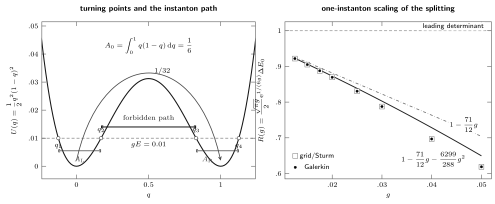
Left: the fixed potential $U(q)=q^2(1-q)^2/2$, its four sub-barrier turning points, equal well regions, and the open barrier path. Right: independently refined parity splittings compared with the one-instanton exponential and its displayed fluctuation corrections; the asymptotic curves are not finite-$g$ equalities.

Near degeneracy makes a small absolute energy error a potentially large relative splitting error. Parity blocks are therefore solved separately, and agreement of two total energies is not accepted as evidence for agreement of their difference. The calculation remains ordinary floating-point linear algebra: it validates the displayed regime, not a uniform error theorem or an interval enclosure.

The low-doublet limit is not uniform

The sub-barrier condition is

$$gE_{\varepsilon,N}<\frac1{32}.$$

For a fixed local level this holds as $g\to0^+$, and a deep-well calculation requires the stronger separation $g(N+\tfrac12)\ll1/32$. It is not legitimate to let $N\sim g^{-1}$ while retaining a fixed-$N$ instanton formula. Near the barrier top, the inner turning points coalesce, the forbidden action shrinks, the nominal doublet is no longer exponentially isolated, and a uniform separatrix analysis replaces the dilute-instanton expansion.

Nor should a finite loop truncation be extrapolated until its bracket changes sign. That sign change diagnoses leaving the asymptotic regime; it does not mean that the exact positive splitting has become negative. The Sturm ordering $E_{+,N}<E_{-,N}$ remains exact.

Common pitfalls

Mixing $E$ with $\mathcal E$. The eigenvalue of $H(g)$ tends to $N+\tfrac12$, while the fixed-potential energy is $\mathcal E=gE$. A turning-point inequality or period written for one cannot be inserted into the other without the factor of $g$.

Doubling the instanton exponent. The open crossing has action $1/6$; the closed barrier cycle has action $1/3$. The boundary determinant uses half the closed dual period for a one-way transition.

Calling half the split the split. The even and odd one-instanton shifts are $\mp\xi$. Their separation is $2\xi$, while the effective hopping matrix element is $t=\xi$ at leading order.

Assigning the perturbative ambiguity to one instanton. One instanton changes wells and controls parity splitting. The perturbative vacuum first couples to the neutral two-event sector, so its leading Borel action is $1/3$.

Dropping the lateral logarithm. Replacing $\log(-2/g)$ by $\log(2/g)$ erases the imaginary contribution needed for ambiguity cancellation. A real median answer is constructed from matched lateral sectors, not by silently editing one formula.

Exercises

1. Cross the normalization dictionary

Starting from $H(g)\psi=E\psi$, recover the fixed-potential equation used for exact WKB and the double-well potential calibrated in Chapter 9.

Solution

Multiplication by $g$ gives

$$\left[ -\frac{g^2}{2}\partial_q^2 +\frac12q^2(1-q)^2 \right]\psi =gE\psi.$$

Set

$$x=-q, \qquad \hbar=g, \qquad \mathcal E=gE.$$

Since $q^2(1-q)^2=x^2(1+x)^2$, the equation becomes

$$\left[ -\frac{\hbar^2}{2}\partial_x^2 +\frac12x^2(1+x)^2 \right]\psi =\mathcal E\psi,$$

which is the Chapter 9 calibration. The coordinate reversal exchanges the two wells but changes neither the spectrum nor the crossing action.

2. Locate the separatrix

Derive the four turning points for $0<\mathcal E<1/32$ and show which pair coalesces at the barrier.

Solution

The equation $U(q)=\mathcal E$ is

$$[q(1-q)]^2=2\mathcal E.$$

With $s=\sqrt{2\mathcal E}$, solve the two quadratics $q(1-q)=s$ and $q(1-q)=-s$. Their roots are

$$q=\frac{1\pm\sqrt{1-4s}}2, \qquad q=\frac{1\pm\sqrt{1+4s}}2.$$

Four real roots require $s<1/4$, equivalently $\mathcal E<1/32$. At equality,

$$q_2=q_3=\frac12,$$

so the two inner roots coalesce at the barrier. The outer roots remain distinct; above the barrier only that outer pair is real.

3. Recover the first local correction

Use harmonic-oscillator perturbation theory near $q=0$ to show that

$$E_N^{(0)}(g) = N+\frac12 -g(3N^2+3N+1) +O(g^2).$$

Solution

With $q=\sqrt g\,y$, use $\lambda=\sqrt g$ and write

$$H=H_0+\lambda V_1+\lambda^2V_2, \qquad V_1=-y^3, \qquad V_2=\frac12y^4.$$

The first-order term in $\lambda$ vanishes by oscillator parity. At order $\lambda^2=g$, the quartic expectation and the second-order cubic sum are

$$\begin{aligned} \langle N|V_2|N\rangle &= \frac38(2N^2+2N+1), \\ \sum_{M\ne N} \frac{|\langle M|y^3|N\rangle|^2}{N-M} &= -\frac18(30N^2+30N+11). \end{aligned}$$

Their sum is $-(3N^2+3N+1)$. For $N=0$, the quartic contribution is $3/8$ and the cubic contribution is $-11/8$, giving the coefficient $-1$.

4. Construct the one-way saddle

Solve the first-order instanton equation, identify its zero mode, and compute its action.

Solution

Separate variables in

$$\dot q=q(1-q): \qquad \frac{\dd q}{q(1-q)}=\dd\tau.$$

Integration gives

$$\log\!\left(\frac{q}{1-q}\right) = \tau-\tau_0,$$

and hence

$$q_I(\tau) = \frac{1}{1+\ee^{-(\tau-\tau_0)}}.$$

Differentiating with respect to $\tau_0$ gives $-\dot q_I$, the translational zero mode of $L_I$. Because the solution saturates the completed square,

$$S_I = \int_0^1q(1-q)\,\dd q = \left[ \frac{q^2}{2}-\frac{q^3}{3} \right]_0^1 = \frac16.$$

5. Read the split from a gamma pole

Expand the generalized quantization condition near $B=N+\tfrac12$ and recover the leading one-instanton shift for the $N$th doublet.

Solution

Use the equivalent branch-resolved inverse-gamma form

$$\frac1{\Gamma(\tfrac12-B_\pm)} + \frac{\pm\varepsilon\ii}{\sqrt{2\pi}} \exp\!\left[ B_\pm\log_\pm\!\left(-\frac2g\right) -\frac12A_\pm \right] =0.$$

Set $B=N+\tfrac12+\delta$. Since

$$\frac1{\Gamma(-N-\delta)} = (-1)^{N+1}N!\,\delta+O(\delta^2),$$

and $A/2=1/(6g)+O(g)$, correlate the upper signs with $\log_+(-2/g)$ and the lower signs with $\log_-(-2/g)$. Both consistent lateral branches give the same leading real displacement. With

$$\Lambda_N(g) := \frac1{N!} \left(\frac2g\right)^N \xi(g),$$

one finds

$$\delta = -\varepsilon\Lambda_N(g) +O\!\left( g\Lambda_N, \Lambda_N^2|\log g| \right).$$

Because $\partial E/\partial B=1+O(g)$, this is also the leading energy shift. Thus

$$\Delta E_N = \frac2{N!} \left(\frac2g\right)^N \xi(g) [1+O(g)].$$

6. Resolve the factor of two

Show that the closed barrier action tends to $1/3$, yet the one-event factor in the boundary determinant is $\exp[-1/(6g)]$.

Solution

At the bottom of the wells, one open passage from $q=0$ to $q=1$ has

$$\int_0^1\sqrt{2U(q)}\,\dd q=S_I=\frac16.$$

A closed contour around the barrier cut has an upper and lower bank. Its classical period is therefore twice the open integral:

$$t_{D,0}=2S_I=\frac13.$$

The parity determinant contains

$$\exp\!\left(-\frac{t_D}{2g}\right),$$

so its classical limit is $\exp[-(1/3)/(2g)]=\exp[-1/(6g)]$. Squaring this event factor produces the neutral scale $\exp[-1/(3g)]$ seen by perturbative large order.

7. Infer the neutral action from coefficients

Starting from a perturbative imaginary part proportional to $-g^{-1}\exp[-1/(3g)]$, derive the leading large-order coefficients and the action estimator.

Solution

The leading dispersion integral is

$$E_{0,k}^{(0)} \sim -\frac1\pi \int_0^\infty g^{-k-2}\ee^{-1/(3g)}\,\dd g.$$

Set $u=1/(3g)$. Reversing the limits gives

$$\int_0^\infty g^{-k-2}\ee^{-1/(3g)}\,\dd g = 3^{k+1}\int_0^\infty u^k\ee^{-u}\,\dd u = 3^{k+1}k!.$$

Therefore

$$E_{0,k}^{(0)} \sim -\frac{3^{k+1}}\pi k!, \qquad k\frac{E_{0,k-1}^{(0)}}{E_{0,k}^{(0)}} \longrightarrow\frac13.$$

No parity label appears because the relevant saddle sequence returns to the well from which it started.

8. Audit an exponentially small doublet

Run the companion program in its default and high-refinement modes. For one coupling, compare the separately computed parity energies, their splitting, and the leading-determinant, $O(g)$, and $O(g^2)$ one-instanton predictions. Explain why agreement of the total energies is insufficient.

Solution

Run

python public/code/advanced-ode/symmetric-double-well-transseries.py
python public/code/advanced-ode/symmetric-double-well-transseries.py --mode high

At the default coupling $g=0.025$, the frozen output is

run/solver	$E_{+,0}$	$E_{-,0}$	$\Delta E_0$
default/Gal.	0.467282072053	0.474825962715	$7.543890662\times10^{-3}$
default/grid	0.467282072068	0.474825962734	$7.543890667\times10^{-3}$
high/Gal.	0.467282072053	0.474825962715	$7.543890662\times10^{-3}$
high/grid	0.467282072054	0.474825962721	$7.543890667\times10^{-3}$

The scaled numerical value is $R=0.83062859$. The leading determinant predicts $R_0=1$; retaining $O(g)$ gives $R_1=0.85208333$; retaining $O(g^2)$ gives $R_2=0.83841363$. The loop corrections move successively toward the numerical value, while the remaining difference measures unshown loops and exponentially smaller odd-event sectors.

The default and high cross-method relative splitting gaps are $6.417\times10^{-10}$ and $6.015\times10^{-10}$. On the grid side, the reported splitting shift under the final refinement decreases from $7.126\times10^{-9}$ to $2.425\times10^{-9}$. These are empirical floating-point diagnostics, not enclosures.

The two parity eigenvalues share many leading digits, so an absolute error that is harmless for either total energy can be comparable with their difference. Separate parity blocks prevent numerical mixing of the near-degenerate pair; cutoff and mesh refinements then test distinct error sources. Agreement must be demanded for $\Delta E_0$ and $R(g)$ themselves, not inferred from matching rounded values of $E_{+,0}$ and $E_{-,0}$.

References

• J. Zinn-Justin and U. D. Jentschura, “Multi-Instantons and Exact Results I: Conjectures, WKB Expansions, and Instanton Interactions”, Annals of Physics 313 (2004), 197–267, arXiv:quant-ph/0501136. Equations (2.10)–(2.27) fix the operator, parity, transseries, generalized quantization condition, and leading splitting used here.
• U. D. Jentschura and J. Zinn-Justin, “Higher-Order Corrections to Instantons”, Journal of Physics A 34 (2001), L253–L258, arXiv:math-ph/0103010. Gives the higher-loop one- and two-instanton coefficients and their numerical tests.
• J. Zinn-Justin and U. D. Jentschura, “Multi-Instantons and Exact Results II: Specific Cases, Higher-Order Effects, and Numerical Calculations”, Annals of Physics 313 (2004), 269–325, arXiv:quant-ph/0501137. Section 8.4 tabulates the fluctuation coefficients through high order.
• E. Delabaere, H. Dillinger, and F. Pham, “Exact Semiclassical Expansions for One-Dimensional Quantum Oscillators”, Journal of Mathematical Physics 38 (1997), 6126–6184. Establishes the sectorial exact-WKB and Borel-resummed foundation of the Zinn-Justin quantization structure for analytic one-dimensional oscillators.
• G. V. Dunne and M. Ünsal, “Uniform WKB, Multi-Instantons, and Resurgent Trans-Series”, Physical Review D 89 (2014), 105009, arXiv:1401.5202. Derives the double-well transseries from uniform WKB and a global parity condition.
• A. van Spaendonck and M. Vonk, “Exact Instanton Transseries for Quantum Mechanics”, SciPost Physics 16 (2024), 103, arXiv:2309.05700. Gives the lateral period quantization and the full, minimal, and median transseries for the symmetric double well.
• B. Simon, “Semiclassical Analysis of Low Lying Eigenvalues II: Tunneling”, Annals of Mathematics 120 (1984), 89–118, and B. Helffer and J. Sjöstrand, “Multiple Wells in the Semi-Classical Limit I”, Communications in Partial Differential Equations 9 (1984), 337–408. These works provide rigorous action-controlled tunneling and multiwell interaction theory; the explicit loop coefficients above are model-specific resurgent data.
• A. Garg, “Tunnel Splittings for One-Dimensional Potential Wells Revisited”, American Journal of Physics 68 (2000), 430–437, arXiv:cond-mat/0003115. Reconciles WKB and instanton prefactors for low-lying double-well splittings.

Here two $L^2$ endpoint conditions, reflection parity, and four finite sub-barrier turning points fixed the spectrum. Page 4 keeps real-line decay but replaces polynomial tails by a real cosh potential. After an exponential coordinate change, the two ends become the irregular singularities of a doubly confluent Heun realization. That modified-Mathieu problem is confining, not the periodic Mathieu operator of Page 2; its precise scalar reduction and Painlevé degeneration belong to the next page.