How to Use This Book

This is a book with one common analytic trunk and several research paths. Read Chapters 1–4 in order unless you already work comfortably with complex singularities, normalized solution bases, monodromy and Stokes data, Wronskians, and recurrence asymptotics. After that, follow the branch that matches the global datum you need.

The shortest useful route

If you arrived with a specific equation, begin with the book overview, read Chapters 1–4, and then jump to the relevant application in Chapter 14 or 15. That application points back to the advanced framework pages it actually uses.

Choose a reading path

The sequences below list principal chapters, not every useful cross-reference. “As relevant” means that the application must first satisfy the hypotheses and normalization dictionary of the method.

Reader or problem	Core path	Main payoff
Special functions and analytic ODEs	Start $\to$ 1–4 $\to$ 5–7 $\to$ 15	Connection matrices, Heun-class equations, recurrence checks, monodromy, and conformal-block formulae
Exact WKB and quantum mechanics	Start $\to$ 1–4 $\to$ 8–10 $\to$ 12–14	Turning-point geometry, resurgent periods, exact quantization, spectral determinants, and tunnelling
CFT and gauge theory	Start $\to$ 1–3 $\to$ 5–7 $\to$ 10–11 $\to$ 15	BPZ equations, accessory parameters, $c=1$ tau expansions, classical blocks, and AGT dictionaries
Black holes and holography	Start $\to$ 1–7 $\to$ 10–13 as relevant $\to$ 15	Horizon-to-boundary connection data, QNMs, response functions, and method selection
Full research path	Read in numerical order	A unified view of direct, monodromic, WKB, gauge-theoretic, and integrable methods

The second route can omit Chapter 11 unless an AGT translation is required. The third route still needs the WKB material when quantum periods or resummation enter. The black-hole route is deliberately conditional: not every separated wave equation has a complete SW/NS, ODE/IM, or TBA description.

Chapter dependencies

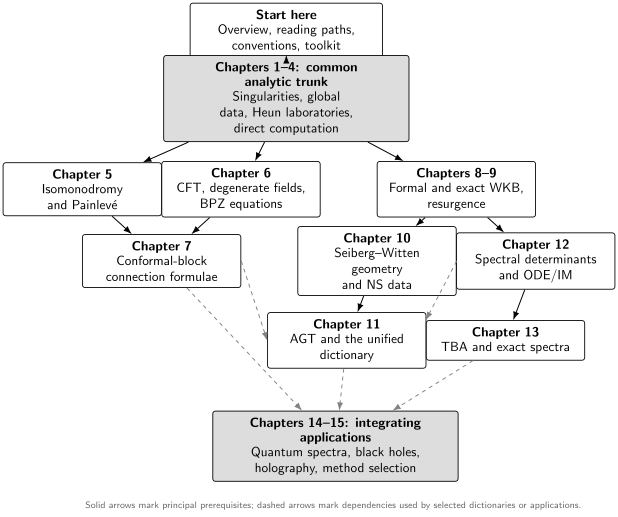
The main prerequisite graph. Solid arrows indicate the normal learning order; dashed arrows indicate dependencies used only by selected dictionaries or applications.

Some dependencies deserve emphasis:

• Chapter 7 assumes both isomonodromy from Chapter 5 and BPZ/conformal-block language from Chapter 6.
• Chapter 10 assumes the spectral curves, cycles, and quantum periods of Chapters 8–9.
• Chapter 11 assumes both the CFT branch and the Seiberg–Witten/NS branch.
• Chapter 13 assumes exact WKB plus the spectral-determinant and functional relation language of Chapter 12.
• Chapters 14–15 use only those branches whose dictionaries have been established for the named model.

The arrows are prerequisites, not assertions that two theories are equivalent. In particular, isomonodromic, CFT, gauge-theory, and integrability objects encode selected ODE data only after their maps and analytic hypotheses have been fixed.

Read each page at three depths

Every conceptual page is designed to support three passes.

1. Orientation pass. Read the lead, assumptions, principal result, interpretation, and worked micro-example. This establishes what the method computes and when it applies.
2. Derivation pass. Work through the displayed equations, limiting checks, and the derivation exercise. Keep the equation and basis conventions in view.
3. Research pass. Audit the normalization ledger, mathematical status, exceptional cases, provenance, and independent checks. Follow the deeper references or reproduce the numerical comparison.

On a first reading, it is reasonable to postpone long calculations. It is not safe to postpone assumptions, branches, basis normalizations, or status labels: those determine what a formula means.

Use the normalization ledger

A substantial connection, monodromy, WKB, or dictionary formula is accompanied by a ledger recording as many of the following as apply:

Ledger entry	Why it matters
Equation and parameter convention	Names such as “HeunC” or “Mathieu” do not fix a unique parameter tuple
Standard and normal forms	Gauge and coordinate changes alter exponents, potentials, and apparent singularities
Local or sectorial bases	Connection coefficients change when either basis is rescaled or mixed
Branches and continuation path	Analytic continuation depends on the homotopy class and branch choices
Wronskian convention	Reversing $W[f,g]=fg'-f'g$ changes signs in determinant formulae
Resonance exclusions	Integer exponent differences may introduce logarithms and singular limiting formulae
Stokes chamber and lateral sum	Exact-WKB quantities depend on $\arg\hbar$, summation direction, and wall-crossing chamber
Cycle orientation and pairing	Quantum periods and gauge-theory periods change sign or basis under cycle transformations
Status and provenance	A formal identity, conditional theorem, and conjectural correspondence make different claims

When comparing two sources, do not compare final formulas first. Compare their ledgers. Many apparent disagreements are basis changes, branch changes, mass shifts, or different definitions of the accessory parameter.

Interpret the status labels

The labels are part of the mathematics, not editorial decoration.

• A theorem includes explicit hypotheses.
• A derivation is established on the page from previously stated results.
• A formal identity concerns formal series and need not define an analytic function.
• A conditional exact statement is exact once its summability, analyticity, topological, and boundary assumptions are satisfied.
• A conjectural correspondence is not silently promoted to a theorem by successful numerical tests.
• A numerical observation records enough information to reproduce the comparison and distinguish empirical accuracy from proof.

For example, an all-orders WKB period is initially formal. A lateral Borel-resummed period is analytic only after a direction and summability statement are supplied. An exact quantization condition additionally requires the turning-point topology, Stokes chamber, and physical boundary conditions.

Work examples before correspondences

Each modern framework is paired with a direct control calculation whenever possible. A reliable order is:

1. identify the canonical local or sectorial bases;
2. express the desired datum as a Wronskian, connection coefficient, or boundary function;
3. compute it by continuation, recurrence, or numerical integration;
4. translate the problem into the advanced framework;
5. compare in an exactly solvable, confluent, symmetry, or high-precision limit.

This order prevents a correspondence from hiding the original boundary-value problem. It also shows whether a tau function, conformal block, quantum period, or spectral determinant supplies the full connection coefficient or only one ingredient.

Check your prerequisites

You are ready for the common trunk if you can do most of the following:

• turn a scalar second-order ODE into a first-order system;
• compute a Wronskian and use Abel’s identity;
• distinguish a pole, branch point, ordinary point, and regular singular point;
• solve a nonresonant Frobenius indicial problem;
• continue a chosen logarithm or power along a specified path;
• track a matrix under a change of basis;
• interpret an asymptotic expansion without assuming convergence;
• formulate an eigenvalue problem as two boundary conditions on a linear ODE.

The just-in-time toolkit supplies concise reviews of fundamental groups, local systems, Riemann surfaces, homology and intersection pairings, and the minimum operator theory needed later. Chapter 1 reviews the ODE items, so imperfect recall is not a reason to delay starting.

Background introduced inside the book

No prior course in Painlevé equations, CFT, supersymmetric gauge theory, resurgence, or integrable models is assumed. Those subjects are developed to the depth required by the connection problem, not as independent surveys.

Exercises and computational labs

Exercises have four recurring levels:

1. Concept check — definitions, transformations, and interpretation.
2. Derivation — a nontrivial identity, limiting case, or basis-change calculation.
3. Computational lab — a high-precision result with a required independent check.
4. Research problem — an open-ended extension whose known and unknown parts are stated explicitly.

Hints appear next to the exercise when they improve learning. Full solutions are separately linkable so that they can be consulted without crowding the argument.

Every computational lab records:

• software and version;
• working precision and target accuracy;
• branches, contours, and initial data;
• convergence or stopping criterion;
• comparison target;
• enough code or pseudocode to reproduce the result.

Ordinary high-precision arithmetic is described as such. The word “certified” is reserved for validated interval or ball computations with a stated enclosure.

A practical study rhythm

For self-study, one conceptual page plus its exercises is a natural session. A chapter typically supports this cycle:

1. read the overview and inspect the chapter’s canonical examples;
2. work through the theory pages in sidebar order;
3. reproduce one derivation without looking;
4. complete the computational lab and its independent check;
5. return to the overview and explain the chapter’s output in connection-data language.

For a course, Chapters 1–4 form a self-contained analytic ODE module. Chapters 8–9 plus Chapter 14 form an exact-WKB and quantum-spectra module. Chapters 5–7 form a monodromy/CFT module. The later gauge and integrability chapters are best taught after one of those modules rather than as isolated dictionaries.

Orientation references

• NIST DLMF, Differential equations and singularity classification, is a concise checkpoint for Frobenius theory, irregular singularities, and Liouville–Green approximation.
• G. Teschl, Mathematical Methods in Quantum Mechanics, provides an author-hosted route into the spectral theory used in Chapters 2 and 14.
• K. Iwasaki, H. Kimura, S. Shimomura, and M. Yoshida, From Gauss to Painlevé, provides a deeper route through Fuchsian equations, monodromy, and isomonodromy.