Quasi-Exact Solvability versus Generic Exact-WKB Behavior

At an integer Razavy parameter, a finite Jacobi matrix returns the first few energies exactly. Move the parameter by any nonzero amount and that matrix immediately loses its invariant-space meaning. The physical Hamiltonian does not disappear: its parity sectors, simple eigenvalues, recessive solutions, and boundary determinants all remain. Away from discriminants, its distinct turning points and exact-WKB connection problem remain as well.

This page makes that separation quantitative. The recurrence shows exactly where the finite polynomial factorization breaks. The boundary determinant shows why each algebraic energy nevertheless continues through the detuning. A one-state example then catches a particularly tempting error: at $\zeta=1$, continuing the frozen finite block predicts the wrong sign for the ground-state slope.

First reading

Follow critical polynomial → detuning leakage → continued determinant zero → the $M=1$ checksum → the comparison table. The local determinant factorization and chamberwise exact-WKB passport can be saved for a second reading.

Status ledger

Statement on this page	Status
$M=m\in\mathbb N$ closes the Razavy polynomial space	Exact algebraic statement in the Page 5 convention
$\Pi_m$ divides all later recurrence polynomials at $M=m$	Exact consequence of the vanished recurrence coefficient
Any $\delta\ne0$ destroys that divisibility and the invariant wall	Exact detuning identity
A simple algebraic level continues with $M$	Local analytic perturbation theorem
The $M=1$ slope in terms of $K_1/K_0$	Exact Hellmann–Feynman calculation
A coordinate-grid slope	Numerical approximation with mesh and detuning errors
Exact-WKB periods and determinants away from QES	Exact only under the Chapter 9 summability, chamber, endpoint, and continuation passport

Two notions of exactness live on different parameter sets

Keep the Page 5 units for the hyperbolic Razavy family,

$$H(M,\zeta) = -\frac{\dd^2}{\dd x^2} + \left( \zeta\cosh2x-M \right)^2, \qquad \zeta>0, \quad M\in\mathbb R.$$

For every real $M$, this is a confining, parity-invariant real-line operator. Its spectrum is discrete and simple,

$$E_0(M)<E_1(M)<E_2(M)<\cdots,$$

and the eigenfunctions alternate even and odd. Integer $M$ adds a finite algebraic structure; it does not create the operator or its boundary problem.

Question	Quasi-exact solvability	Exact WKB
Where does it live?	Special algebraic slices of coupling space	Open graph chambers, with lateral data on their walls
Central object	A finite invariant space and characteristic polynomial	Borel-summed local solutions, Voros symbols, and a boundary determinant
What is obtained?	Finitely many exact energies and eigenfunctions	Exact connection or quantization data in the declared analytic domain
Does it give the full spectrum?	No, except in a genuinely finite problem	In principle yes for the boundary problem covered by the determinant
Must the answer be elementary?	The roots may still require algebraic or numerical evaluation	No; exact Borel sums often require numerical evaluation
What fails under generic detuning?	The invariant wall and finite characteristic polynomial	Data persist; discriminants change local models and covered Stokes walls change charts

“Exact” therefore modifies different nouns. QES makes a finite restriction exact. Exact WKB makes a connection identity exact after its summability and continuation hypotheses have been proved.

One vanished recurrence coefficient creates the critical polynomial

Reuse the monic Razavy energy polynomials from Page 5:

$$\Pi_{-1}=0, \qquad \Pi_0=1,$$

and

$$\Pi_{k+1} = \left(E-b_k\right)\Pi_k -a_k\Pi_{k-1},$$

where

$$\begin{aligned} a_k &= 4\zeta^2k(M-k), \\ b_k &= 4k(M-1-k)+2M-1+\zeta^2. \end{aligned}$$

These formal polynomials can be generated for arbitrary real $M$. Their QES meaning appears only when $M=m\in\mathbb N$. Then

$$a_m=0,$$

so the first row beyond the finite block reads

$$\Pi_{m+1} = \left(E-b_m\right)\Pi_m.$$

Every later polynomial inherits the same factor:

$$\Pi_{m+\ell}(E) = \Pi_m(E)Q_\ell(E), \qquad \ell=0,1,2,\ldots.$$

The proof is induction in the three-term recurrence. The degree-$m$ factor $\Pi_m$ is the critical polynomial. Its $m$ simple roots are the eigenvalues of the symmetric QES Jacobi block and, for this real-line Razavy problem, exactly the first $m$ physical levels.

Strictly, the invariant wavefunction space is the Page 5 gauge factor times $\mathcal P_{m-1}$. The gauge restores decay at both real ends; finite polynomial invariance by itself would not prove normalizability in a generic QES model.

The later factorization is an algebraic fingerprint of the invariant wall. It does not turn the infinite-dimensional boundary determinant into a polynomial. At $M=m$, all levels above $E_{m-1}$ still require the full connection problem.

Detuning reopens the recurrence wall

Set

$$M=m+\delta.$$

The formerly vanished coefficient becomes

$$a_m = 4\zeta^2m\delta.$$

Consequently,

$$\begin{aligned} \Pi_{m+1} ={}& \left(E-b_m\right)\Pi_m \\ &- 4\zeta^2m\delta\,\Pi_{m-1}. \end{aligned}$$

At a root of $\Pi_m$, the right side is generically nonzero as soon as $\delta\ne0$. Critical-polynomial divisibility is lost to first order in the detuning.

The same obstruction is visible before the recurrence is formed. With the Page 5 gauge, the polynomial space at the integer point is

$$\mathcal P_{m-1} = \operatorname{span} \{1,r,\ldots,r^{m-1}\}.$$

If that space is kept fixed while $M=m+\delta$, the gauged Hamiltonian sends its highest monomial to

$$\mathcal H_g r^{m-1} = -2\zeta\delta\,r^m + \text{terms in }\mathcal P_{m-1}.$$

The coefficient of $r^m$ is not a small correction inside the finite matrix; it points outside the proposed invariant space. Truncating that row by hand produces a numerical finite section, not a detuned QES Hamiltonian.

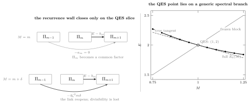
Left: at $M=m$, $a_m=0$ isolates the critical polynomial $\Pi_m$; detuning reopens the link with strength $4\zeta^2m\delta$. Right: for $\zeta=1$, the full ground-state branch passes smoothly through the exact QES point $(M,E)=(1,2)$. Its true tangent has negative slope, whereas a frozen $1\times1$ block gives the spurious slope $+2$.

The boundary determinant survives after the polynomial disappears

Let $u_R(x;E,M)$ be the right-recessive solution, with any fixed analytic asymptotic normalization. Reflection symmetry converts the two-ended problem into the parity determinants

$$\begin{aligned} D_+(E,M) &= u_R'(0;E,M), \\ D_-(E,M) &= u_R(0;E,M). \end{aligned}$$

Their zeros are respectively the even and odd eigenvalues. Multiplying $u_R$ by a nowhere-vanishing analytic factor changes neither zero set. With the reflection-related left normalization, the full two-ended Wronskian factorizes as

$$\Wr\!\left[u_R(-x),u_R(x)\right] = 2D_-(E,M)D_+(E,M).$$

This identity connects the parity test at the origin to the global left–right boundary determinant used by exact WKB.

At $M=m$, reversal parity splits the critical polynomial:

$$\Pi_m = \Pi_{m,+}\Pi_{m,-}.$$

The roots of $\Pi_{m,+}$ are the algebraic even levels and those of $\Pi_{m,-}$ are the algebraic odd levels. In a neighborhood containing those roots but no higher eigenvalue, simplicity gives the local factorization

$$D_p(E,m) = U_p(E)\Pi_{m,p}(E), \qquad p=\pm,$$

where $U_p$ is analytic and nowhere zero there. This is a factorization of the local zero divisor, not a claim that $D_p$ is globally polynomial: each $D_p$ has infinitely many additional zeros.

For $\delta\ne0$, $\Pi_{m,p}$ ceases to be a finite spectral factor, but $D_p(E,m+\delta)$ remains the boundary function. If $D_p(E_\star,m)=0$ is simple, the implicit-function theorem produces a unique nearby branch,

$$D_p(E(M),M)=0,$$

with

$$\left. \frac{\dd E}{\dd M} \right|_{M=m} = - \left. \frac{\partial_M D_p} {\partial_E D_p} \right|_{(E_\star,m)}.$$

Thus an algebraic energy does not vanish under detuning. Only its finite formula vanishes.

Expert check: why the real branches are analytic

The leading tail $\zeta^2\cosh^2 2x$ is independent of $M$. On any bounded $M$-interval, the perturbation

$$-2\zeta M\cosh2x+M^2$$

is form-bounded with arbitrarily small relative bound against that tail. The closed quadratic forms therefore constitute a local analytic family. Every one-dimensional eigenvalue is simple, so analytic perturbation theory gives a single real-analytic branch rather than a branching eigenvalue cluster.

For a normalized eigenfunction, differentiating the operator gives the equivalent Hellmann–Feynman formula

$$\frac{\dd E_n}{\dd M} = 2\int_{\mathbb R} \left( M-\zeta\cosh2x \right) \lvert\psi_n(x;M)\rvert^2\,\dd x.$$

The determinant derivative and the expectation value compute the same spectral slope in two different representations.

The one-state slice exposes a fake finite-block continuation

At $M=1$, the invariant space consists only of the constant polynomial. The normalized algebraic ground state and its energy are

$$\begin{aligned} \psi_0(x;1) &= \frac{ \exp[-\zeta\cosh(2x)/2] }{ \sqrt{K_0(\zeta)} }, \\ E_0(1) &= \zeta^2+1. \end{aligned}$$

The normalization follows from the standard integral representation

$$K_\nu(\zeta) = \int_0^\infty \ee^{-\zeta\cosh t} \cosh(\nu t)\,\dd t.$$

Hellmann–Feynman now gives an exact tangent to the generic ground-state branch:

$$\boxed{ E_0'(1) = 2\left[ 1-\zeta \frac{K_1(\zeta)}{K_0(\zeta)} \right]. }$$

By contrast, if one freezes the $1\times1$ block and merely substitutes a noninteger $M$ into its diagonal entry,

$$b_0(M)=2M-1+\zeta^2,$$

the predicted slope is $2$. The missing term $-2\zeta K_1/K_0$ is precisely the effect of the wavefunction outside the false one-dimensional truncation.

For $\zeta=1$:

Audit quantity	Value
Exact QES energy $E_0(1)$	$2$
Exact analytic slope $E_0'(1)$	$-0.8592507965\ldots$
Centered grid slope with $\delta=10^{-2}$	$-0.8592531$
Frozen-block slope	$+2$

The coordinate value comes from Richardson-refined parity grids at $M=1-\delta$, $1$, and $1+\delta$. Agreement with the exact tangent tests both the detuning calculation and the generic real-line solver; the frozen-block result fails even qualitatively.

The NumPy-only companion program razavy-qes-detuning.py reproduces the table and the curve in the figure. Run

python3 public/code/advanced-ode/razavy-qes-detuning.py
python3 public/code/advanced-ode/razavy-qes-detuning.py \
  --profile high --csv /tmp/razavy-qes-detuning.csv

The CSV records all eleven curve points, fine-grid values, refinement shifts, Sturm widths, the analytic and centered slopes, and all grid and quadrature settings. The high profile is a refinement check, not a promise that floating-point error decreases monotonically.

What this checksum proves

The Bessel formula is an exact first derivative at one QES point. It does not supply a closed form for $E_0(M)$ at finite detuning. The grid values approximate that continued branch; they do not promote it to another algebraic sector.

Exact-WKB data do not require the integer slice

For the physical comparison, take $M>0$ and restore a positive kinetic parameter $\hbar>0$:

$$H_\hbar = -\hbar^2\frac{\dd^2}{\dd x^2} + \left( \zeta\cosh2x-M \right)^2.$$

Dividing by $\hbar^2$ returns the Page 5 form with

$$\widetilde\zeta=\frac{\zeta}{\hbar}, \qquad \widetilde M=\frac{M}{\hbar}, \qquad \widetilde E=\frac{E}{\hbar^2}.$$

The algebraic slice is therefore

$$\frac{M}{\hbar}=m\in\mathbb N.$$

At fixed physical $M$, the calibration values

$$\hbar_m=\frac{M}{m}, \qquad m=1,2,\ldots,$$

accumulate at the semiclassical endpoint while the invariant-space dimension grows. In Page 6’s double-well normalization, where

$$\begin{aligned} \eta &= \frac{\hbar}{a(M-\zeta)}, & C &= \frac{M}{\zeta}>1, \\ a &= \frac12\operatorname{arcosh}C. \end{aligned}$$

the same sequence is

$$\eta_m = \frac{C}{a(C-1)m},$$

This inverse-integer sequence supplies exact anchors inside the WKB family, not a sequence at which the WKB recursion terminates.

This arithmetic hypersurface is not a turning-point discriminant. For generic $M/\hbar$, the leading spectral curve in $r=\ee^{2x}$ remains

$$Y^2 = \left[ \zeta(r^2+1)-2Mr \right]^2 -4Er^2,$$

with WKB differential

$$\lambda = \frac{Y}{4r^2}\,\dd r.$$

Writing the quartic right side of the curve as $P_4(r)$, its exact discriminant is

$$\begin{aligned} \operatorname{Disc}_r P_4 ={}& 4096E^2\zeta^4 \\ &\times \left[(M-\zeta)^2-E\right] \left[(M+\zeta)^2-E\right]. \end{aligned}$$

Integer $M/\hbar$ is absent from this condition. A generic QES point lies on a smooth genus-one curve.

Away from collisions and unaccounted Stokes walls, the following data continue with the parameters:

• the turning points on the chosen cover;
• a Gauss–Manin-transported cycle and path basis;
• regularized formal quantum periods;
• their directional or lateral Borel sums;
• the two recessive endpoint lines;
• the exact-WKB boundary determinant.

What may change is their coordinate formula. A Stokes wall acts on Voros symbols and connection matrices, while the physical zero divisor is continued covariantly. A discriminant instead changes the local turning model and may require Weber or a higher uniform approximation.

For orientation, distinct special loci include

Locus	What happens	Is it QES?
$M/\hbar=m\in\mathbb N$	A finite recurrence wall closes	Yes
$E=0$	Pairs of turning points coincide at zeros of the squared potential	Not in general
$E=(M-\zeta)^2$, $r=1$	Collision at the real central stationary point	Not in general
$E=(M+\zeta)^2$, $r=-1$	Collision at the complex stationary point	Not in general
A Stokes wall	The active graph and Voros chart change	Not in general

For example, at $(\zeta,M,\hbar)=(1,4,1)$ the algebraic energies are $6$, $14-4\sqrt3$, $14$, and $14+4\sqrt3$, while the discriminant energies are $0$, $9$, and $25$. None of the QES levels degenerates the curve. The first two have four real turning points and the last two only the outer real pair, so one finite algebraic block even straddles two WKB topologies.

Expert checkpoint: periods are transported, not frozen

Let

$$p(x;E,M) = \sqrt{ (\zeta\cosh2x-M)^2-E }.$$

The branch-difference WKB form begins

$$\Omega(\hbar) = \left[ p + \hbar^2 \left( \frac{p''}{4p^2} - \frac{3(p')^2}{8p^3} \right) + O(\hbar^4) \right]\dd x.$$

No coefficient vanishes merely because $M/\hbar$ is an integer. On a discriminant-free patch, transport $\gamma(E,M)$ by the Gauss–Manin connection and set $Z_\gamma=\oint_\gamma p\,\dd x$. Then

$$\begin{aligned} \partial_M Z_\gamma &= \oint_\gamma \frac{M-\zeta\cosh2x}{p}\,\dd x, \\ \partial_E Z_\gamma &= -\frac12 \oint_\gamma \frac{\dd x}{p}. \end{aligned}$$

For a vanishing cycle, the displayed Gauss–Manin chart becomes singular at the collision; unaffected cycles may still be continued in another basis. Across a Stokes wall, the lateral Voros coordinates wall-cross; the analytically continued boundary zero divisor remains the invariant object.

In any domain where the Chapter 9 exact-WKB passport is satisfied, the summed WKB determinant equals the analytic boundary determinant up to a nowhere-zero factor. At an integer slice it must reproduce every algebraic zero in its domain, but its formal WKB series does not thereby terminate. At a noninteger slice it continues to encode the spectrum even though no finite polynomial factor exists.

Evaluation at the physical value of $\hbar$ still requires justified summation or analytic continuation. “Generic” means that QES arithmetic is unnecessary; it does not mean that all exact-WKB hypotheses become automatic. In particular, $\arg\hbar$, the Borel direction, graph chamber, cover and cycle basis, endpoint normalizations, and continuation path must all be fixed.

Use the overlap as a calibration protocol

The QES and exact-WKB descriptions overlap most productively when they are kept independent:

1. Fix the operator, parity sector, endpoint normalization, and parameter convention.
2. On $M=m$, verify both closure and $\Pi_m(E)=0$.
3. Check the algebraic roots against a parity-resolved coordinate solver.
4. Construct the exact-WKB boundary determinant with its chamber and lateral prescription.
5. Require that it reproduce the same simple zeros without tuning a zero-producing normalization factor.
6. Detune $M$ and continue the determinant zero; do not continue the finite matrix.
7. Track recurrence leakage, mesh refinement, WKB truncation or Borel–Padé stability, and distance to discriminants as separate diagnostics.

Page 5 supplied the finite recurrence and direct numerical baselines. The next page, Three controlled capstones, adds exact WKB as an independent third calculation and applies the same discipline to modified Mathieu and anharmonic-oscillator spectra.

Common pitfalls

Continuing the size of a matrix to noninteger values. A matrix dimension is not an analytic parameter. Freeze an integer space and the detuned gauged operator leaks out of it; round the dimension and the result becomes an arbitrary cutoff.

Treating a critical polynomial as the full spectral determinant. $\Pi_m$ contains only the first $m$ Razavy levels. The parity determinants retain infinitely many higher zeros at the same integer parameter.

Expecting WKB to terminate at a QES point. The finite polynomial is a property of a gauged recurrence. Exact WKB is an all-orders connection construction, and its formal series generally remains divergent and in need of summation.

Calling a numerical root exact because it agrees with QES. Agreement calibrates the implementation. The numerical value still carries domain, mesh, precision, and root-finding errors.

Dragging one Voros formula through every parameter value. Turning points can collide and Stokes graphs can wall-cross. Continue the full boundary problem with its chart changes, not one frozen symbolic expression.

Exercises

1. Prove critical-polynomial divisibility

At $M=m\in\mathbb N$, prove that $\Pi_m$ divides every $\Pi_{m+\ell}$.

Solution

Because $a_m=0$,

$$\Pi_{m+1} = (E-b_m)\Pi_m,$$

so the assertion holds for $\ell=0,1$. Suppose

$$\Pi_{m+j}=\Pi_mQ_j, \qquad \Pi_{m+j-1}=\Pi_mQ_{j-1}.$$

The recurrence gives

$$\begin{aligned} \Pi_{m+j+1} &= (E-b_{m+j})\Pi_{m+j} -a_{m+j}\Pi_{m+j-1} \\ &= \Pi_m \left[ (E-b_{m+j})Q_j -a_{m+j}Q_{j-1} \right]. \end{aligned}$$

Thus the factor persists by induction. The proof uses the invariant-wall condition $a_m=0$; a root of $\Pi_m$ alone would not establish it.

2. Quantify the detuning leak

Put $M=m+\delta$. Derive the first row that breaks divisibility and explain why deleting it is not perturbation theory.

Solution

At $k=m$,

$$a_m = 4\zeta^2m(M-m) = 4\zeta^2m\delta.$$

Hence

$$\Pi_{m+1} = (E-b_m)\Pi_m -4\zeta^2m\delta\,\Pi_{m-1}.$$

Even if $\Pi_m(E)=0$, the last term is generically nonzero. In the gauged operator the same change produces

$$\mathcal H_g r^{m-1} = -2\zeta\delta r^m + \text{lower powers}.$$

The omitted vector $r^m$ belongs to the complement of $\mathcal P_{m-1}$. Deleting it changes the operator instead of expanding the true eigenpair.

3. Factor only the local zero divisor

Let $\Pi_{m,p}$ contain the simple algebraic roots of parity $p$, and let $D_p(E,m)$ be analytic with the same roots. Prove the local factorization $D_p=U_p\Pi_{m,p}$ and explain why $U_p$ cannot be declared globally zero-free.

Solution

Near a root $E_j$, both functions have a simple zero, so

$$\frac{D_p(E,m)}{\Pi_{m,p}(E)}$$

has a removable singularity with a nonzero limiting value. Removing all such singularities in a neighborhood of the algebraic roots defines an analytic, nowhere-zero $U_p$ there.

Globally, $D_p$ has the infinitely many nonalgebraic parity levels as additional zeros, whereas $\Pi_{m,p}$ is finite degree. Their quotient therefore vanishes at higher levels. The zero-free assertion is local to a domain that excludes those levels.

4. Continue a simple determinant zero

Starting from $D_p(E(M),M)=0$, derive the determinant formula for $E'(M)$. Then derive the Hellmann–Feynman expression directly from the normalized eigenvalue equation.

Solution

Differentiation of the scalar equation gives

$$\partial_E D_p\,E'(M)+\partial_M D_p=0.$$

At a simple zero $\partial_ED_p\ne0$, so

$$E'(M) = -\frac{\partial_MD_p}{\partial_ED_p}.$$

For $H\psi=E\psi$ with $\langle\psi,\psi\rangle=1$, differentiate and take the inner product with $\psi$. Self-adjointness cancels the terms involving $\psi'$, leaving

$$E'(M) = \left\langle\psi,\partial_MH\,\psi\right\rangle.$$

Since

$$\partial_MH = 2(M-\zeta\cosh2x),$$

this is the integral displayed in the text.

5. Derive the one-state tangent

Verify the $M=1$ eigenpair, normalize it, and compute $E_0'(1)$.

Solution

For

$$\psi(x)=\exp[-\zeta\cosh(2x)/2],$$

direct differentiation gives

$$\left[ -\partial_x^2 + (\zeta\cosh2x-1)^2 \right]\psi = (\zeta^2+1)\psi.$$

With $t=2x$ and evenness,

$$\int_{-\infty}^{\infty} \ee^{-\zeta\cosh2x}\,\dd x = \int_0^\infty \ee^{-\zeta\cosh t}\,\dd t = K_0(\zeta).$$

Similarly,

$$\left\langle\cosh2x\right\rangle = \frac{K_1(\zeta)}{K_0(\zeta)}.$$

Substitution into Hellmann–Feynman yields

$$E_0'(1) = 2\left[ 1-\zeta\frac{K_1(\zeta)}{K_0(\zeta)} \right].$$

At $\zeta=1$, this is $-0.8592507965\ldots$, not $+2$.

6. Restore the kinetic parameter

Assume $M>0$ and $\hbar>0$. Show that the QES condition for $H_\hbar$ is $M/\hbar\in\mathbb N$. Why does this not impose a turning-point collision?

Solution

Divide the eigenvalue equation by $\hbar^2$:

$$\left[ -\partial_x^2 + \left( \frac{\zeta}{\hbar}\cosh2x -\frac{M}{\hbar} \right)^2 \right]\psi = \frac{E}{\hbar^2}\psi.$$

It is the Page 5 operator with parameters $\widetilde\zeta=\zeta/\hbar$ and $\widetilde M=M/\hbar$. Closure therefore requires $\widetilde M\in\mathbb N$.

Turning collisions are instead zeros of the spectral discriminant, such as $E=0$ or $E=(M\mp\zeta)^2$. The arithmetic condition on $M/\hbar$ does not force any of these energy relations.

7. Design a three-way audit

At $\zeta=1$, $M=4$, specify what recurrence, direct numerics, and exact WKB must each compute. Then state what changes at $M=4+\delta$.

Solution

At the integer point, the recurrence gives the first four levels from $\Pi_4(E)=0$. A parity-resolved coordinate solver must reproduce those four roots and can also compute higher, nonalgebraic levels. An exact-WKB calculation must construct the two parity boundary determinants in a declared chamber and reproduce the same zeros in its validated domain.

At nonzero $\delta$, the finite invariant block and critical polynomial lose their spectral status. The coordinate solver still computes the full real spectrum. The exact-WKB construction still computes the boundary determinants, provided its turning-point and summability passport remains valid; its cycles must be continued and may require a wall-crossed chart. The former QES levels are followed as simple determinant zeros.

References

• M. Razavy, “An exactly soluble Schrödinger equation with a bistable potential,” American Journal of Physics 48 (4) (1980), 285–288, doi:10.1119/1.12141, introduces the hyperbolic model and its finite algebraic sector.
• F. Finkel, A. González-López, and M. A. Rodríguez, “On the families of orthogonal polynomials associated to the Razavy potential,” Journal of Physics A: Mathematical and General 32 (39) (1999), 6821–6835, doi:10.1088/0305-4470/32/39/308, arXiv:math-ph/9905020, develops the critical energy polynomials and invariant sector in this convention.
• A. V. Turbiner, “Quasi-exactly-solvable problems and $\mathfrak{sl}(2)$ algebra,” Communications in Mathematical Physics 118 (1988), 467–474, doi:10.1007/BF01466727, gives the finite-dimensional Lie-algebraic framework for QES operators.
• C. M. Bender and G. V. Dunne, “Quasi-exactly solvable systems and orthogonal polynomials,” Journal of Mathematical Physics 37 (1996), 6–11, doi:10.1063/1.531373, arXiv:hep-th/9511138, develops critical-polynomial factorization and weak orthogonality.
• A. González-López, N. Kamran, and P. J. Olver, “Normalizability of one-dimensional quasi-exactly solvable Schrödinger operators,” Communications in Mathematical Physics 153 (1993), 117–146, doi:10.1007/BF02099042, separates formal invariant modules from physical normalizable sectors.
• T. Kato, Perturbation Theory for Linear Operators, 2nd ed., Springer, 1995, doi:10.1007/978-3-642-66282-9, supplies the analytic-family and simple-eigenvalue continuation framework.
• E. Delabaere, H. Dillinger, and F. Pham, “Exact Semiclassical Expansions for One-Dimensional Quantum Oscillators”, Journal of Mathematical Physics 38 (1997), 6126–6184, supplies the exact-WKB treatment of analytic one-dimensional oscillator spectra.
• K. Iwaki and T. Nakanishi, “Exact WKB analysis and cluster algebras,” Journal of Physics A: Mathematical and Theoretical 47 (2014), 474009, doi:10.1088/1751-8113/47/47/474009, arXiv:1401.7094, treats deformations of meromorphic quadratic differentials and Voros-symbol wall crossing.
• A. Voros, “Exact quantization condition for anharmonic oscillators (in one dimension),” Journal of Physics A: Mathematical and General 27 (1994), 4653–4661, doi:10.1088/0305-4470/27/13/038, gives a primary exact-quantization benchmark without implying a Razavy-specific closed formula.
• NIST Digital Library of Mathematical Functions, §10.32, Integral Representations of Modified Bessel Functions, fixes the $K_\nu$ integral used in the one-state checksum.