Quartic versus Hyperbolic Double Wells

The quartic well and the Razavy well look alike on the real axis: below the barrier, each has two allowed islands separated by an open forbidden path. That resemblance is useful only after the coordinate, barrier height, kinetic scale, and energy have been matched.

Once both minima are placed at $X=\pm1$ and both barriers have height one, the comparison becomes exact:

$$\begin{aligned} v_{\mathrm R}(X;a) &\ge v_{\mathrm Q}(X), \\ v_{\mathrm R}(X;a) &\longrightarrow v_{\mathrm Q}(X) \quad (a\to0). \end{aligned}$$

At a common normalized kinetic scale $\eta$, the first statement orders the indexed eigenvalues. The second gives a controlled local quartic limit of the hyperbolic well, not uniform convergence on $\mathbb R$. Neither statement makes the global ODEs identical: polynomial infinity and the two irregular ends of a DCHE problem retain different Stokes and connection data.

First reading

Follow common passport → ordered shapes → turning points → barrier actions → method choice. The min–max argument, double-scaling limit, and punctured spectral curves are independent expert checkpoints.

Status ledger

Statement	Status and scope
Changes of coordinate and normalization	Exact
Shape inequality, curvatures, turning points, and bottom actions	Exact
Spectral ordering at matched kinetic scale	Exact min–max consequence
Quartic limit of fixed indexed levels	Exact limiting statement at fixed normalized kinetic scale
Narrow-doublet estimates	Fixed-level semiclassical asymptotics
Comparison of splitting exponents	Leading exponential statement; prefactors remain model-specific
Heun labels	Require the displayed exponential coordinate or an affine scaling and gauge
Razavy finite algebra	Exact only when $M\in\mathbb N$ and only for the first $M$ states

One barrier-normalized passport makes comparison meaningful

Use the common spectral problem

$$\mathscr L[v,\eta]\psi = \left( -\eta^2\frac{\dd^2}{\dd X^2} +v(X) \right)\psi = \varepsilon\psi.$$

Here the minima are at $X=\pm1$, the central barrier is $v(0)=1$, and $\eta$ measures kinetic energy relative to the chosen separation and barrier.

For the quartic convention of Page 3, set

$$X=2q-1.$$

Multiplying its eigenvalue equation by $32g$ gives

$$\left[ -(8g)^2\frac{\dd^2}{\dd X^2} +(1-X^2)^2 \right]\psi = 32gE_{\mathrm Q}\psi.$$

For Razavy, write

$$a = \frac12\operatorname{arcosh}\!\left(\frac M\zeta\right), \qquad C=\cosh2a=\frac M\zeta, \qquad X=\frac xa,$$

in the double-well chamber $M>\zeta$. Division by the barrier $(M-\zeta)^2$ gives

$$\left[ -\frac{1}{a^2(M-\zeta)^2} \frac{\dd^2}{\dd X^2} +v_{\mathrm R}(X;a) \right]\psi = \frac{E_{\mathrm R}}{(M-\zeta)^2}\psi,$$

where

$$v_{\mathrm R}(X;a) = \left[ \frac{\cosh2a-\cosh(2aX)} {\cosh2a-1} \right]^2.$$

The dictionary is therefore

Datum	Quartic	Razavy
Shape	$v_{\mathrm Q}=(1-X^2)^2$	$v_{\mathrm R}(X;a)$
Kinetic scale	$\eta_{\mathrm Q}=8g$	$\eta_{\mathrm R}=[a(M-\zeta)]^{-1}$
Energy	$\varepsilon_{\mathrm Q}=32gE_{\mathrm Q}$	$\varepsilon_{\mathrm R}=E_{\mathrm R}/(M-\zeta)^2$
Shape parameter	none	$a=\tfrac12\operatorname{arcosh}(M/\zeta)$

Raw energies or raw barrier actions from the two pages should not be placed in one ratio. A matched comparison means the same $\eta$ in the normalized operators. Choosing $\eta_{\mathrm Q}=\eta_{\mathrm R}$ is a comparison protocol, not a universal identity between $g$ and $(\zeta,M)$.

The normalized hyperbolic shape lies above the quartic

The ordering follows from the power series of $\cosh$. Put $u=X^2$. For $0\le u\le1$,

$$\cosh(2aX)-1 = \sum_{k\ge1} \frac{(2a)^{2k}u^k}{(2k)!} \le u\bigl(\cosh2a-1\bigr),$$

whereas the inequality reverses for $u\ge1$. In both ranges,

$$\frac{ \left|\cosh(2aX)-\cosh2a\right| }{ \cosh2a-1 } \ge \left|X^2-1\right|.$$

Squaring proves

$$v_{\mathrm R}(X;a)\ge v_{\mathrm Q}(X) \qquad (X\in\mathbb R,\ a>0).$$

Equality holds at the barrier and minima, $X=0,\pm1$, but is strict elsewhere. Thus barrier- and separation-matched hyperbolic wells are everywhere no lower than the quartic well.

Their local curvatures sharpen the picture:

$$\begin{array}{c|cc} &X=0&X=\pm1\\ \hline v_{\mathrm Q}'' &-4&8\\ v_{\mathrm R}'' &-\dfrac{4a^2}{\sinh^2a} &8a^2\coth^2a \end{array}$$

For $a>0$, the normalized hyperbolic barrier is flatter at its top and its minima are steeper. Between the three matching points its barrier sits higher.

On every fixed compact set,

$$v_{\mathrm R}(X;a) = (1-X^2)^2 \left[ 1+\frac{2a^2X^2}{3}+O(a^4) \right].$$

The bracketed form means

$$v_{\mathrm R} = v_{\mathrm Q} +\frac{2a^2}{3}X^2(1-X^2)^2 +O(a^4).$$

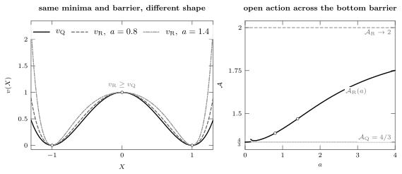
Left: after matching minima and barrier height, the Razavy shapes lie at or above the quartic shape and approach it as $a\to0$. Right: the dimensionless bottom action starts at $\mathcal A_{\mathrm Q}=4/3$ and approaches $2$ as the hyperbolic well becomes increasingly steep away from its minima.

Expert checkpoint: spectral ordering and convergence

At fixed $\eta$, form ordering and the min–max principle give

$$\varepsilon_n^{\mathrm R}(a,\eta) > \varepsilon_n^{\mathrm Q}(\eta), \qquad n=0,1,\ldots.$$

For strictness, put $W=v_{\mathrm R}-v_{\mathrm Q}$ and $W_K=\min(W,K)$ with any $K>0$. The bounded function $W_K$ is positive almost everywhere. Along

$$H_t=H_{\mathrm Q}+tW_K, \qquad 0\le t\le1,$$

one-dimensional bound-state eigenvalues are simple, so the Hellmann–Feynman identity gives

$$\frac{\dd E_n(t)}{\dd t} = \int_{\mathbb R} W_K(X)\lvert\psi_{n,t}(X)\rvert^2\,\dd X >0.$$

Since $H_{\mathrm R}\ge H_{\mathrm Q}+W_K$, a second use of min–max proves the displayed strict inequality for every $n$.

The pointwise limit is not uniform on the whole line: polynomial and exponential tails never become the same at fixed $a$. Nevertheless, for each fixed $n$ and $\eta>0$,

$$\lim_{a\to0^+} \varepsilon_n^{\mathrm R}(a,\eta) = \varepsilon_n^{\mathrm Q}(\eta).$$

The lower bound is the form ordering. For the upper bound, smoothly cut off the first $n+1$ quartic eigenfunctions outside a large compact interval and use uniform convergence of $v_{\mathrm R}$ on that interval in the min–max trial space. The cutoff error is made small before $a\to0$ is taken.

Four real turning points share one separatrix skeleton

Let $0<\varepsilon<1$. For the quartic shape,

$$X_{\mathrm{in}}^{\mathrm Q} = \sqrt{1-\sqrt\varepsilon}, \qquad X_{\mathrm{out}}^{\mathrm Q} = \sqrt{1+\sqrt\varepsilon}.$$

For the hyperbolic shape,

$$\begin{aligned} X_{\mathrm{in}}^{\mathrm R} &= \frac{1}{2a} \operatorname{arcosh}\!\left[ C-(C-1)\sqrt\varepsilon \right], \\ X_{\mathrm{out}}^{\mathrm R} &= \frac{1}{2a} \operatorname{arcosh}\!\left[ C+(C-1)\sqrt\varepsilon \right]. \end{aligned}$$

In either model the ordered real roots are

$$-X_{\mathrm{out}}, \quad -X_{\mathrm{in}}, \quad X_{\mathrm{in}}, \quad X_{\mathrm{out}}.$$

The outer pairs bound two equal allowed intervals; the inner pair bounds the forbidden barrier. At $\varepsilon=1$, the inner roots collide at $X=0$. Above the barrier, only the outer pair remains real. Expanding the hyperbolic formulas at small $a$ recovers the quartic formulas.

Four roots alone do not guarantee a narrow doublet. Near a minimum, the local harmonic energies measured in units of the barrier are

$$\begin{aligned} d_{\mathrm Q,N} &= 2(2N+1)\eta, \\ d_{\mathrm R,N} &= 2a\coth a\,(2N+1)\eta. \end{aligned}$$

The diagnostic $d_N\ll1$ places a fixed local level well below the separatrix. It is not an error bound. When $d_N$ approaches one, the inner turning points coalesce and a uniform Weber (parabolic-cylinder) barrier-top analysis replaces a dilute-instanton expansion.

Equal barriers do not mean equal tunnelling actions

For a barrier-normalized shape define the open bottom action

$$\mathcal A[v] = \int_{-1}^{1}\sqrt{v(X)}\,\dd X.$$

The quartic value is

$$\mathcal A_{\mathrm Q} = \int_{-1}^{1}(1-X^2)\,\dd X = \frac43.$$

For Razavy,

$$\begin{aligned} \mathcal A_{\mathrm R}(a) &= \frac{1}{C-1} \int_{-1}^{1} \left[C-\cosh(2aX)\right]\dd X \\ &= \frac{ 2\cosh2a-\sinh(2a)/a }{ \cosh2a-1 }. \end{aligned}$$

The shape inequality gives

$$\mathcal A_{\mathrm R}(a)>\frac43 \qquad (a>0),$$

and direct expansion yields

$$\begin{aligned} \mathcal A_{\mathrm R}(a) &= \frac43+\frac{4a^2}{45}+O(a^4), \qquad a\to0, \\ \mathcal A_{\mathrm R}(a) &= 2-\frac1a+O(\ee^{-2a}), \qquad a\to\infty. \end{aligned}$$

The normalized exponents reproduce the raw actions on the two earlier pages:

$$\frac{\mathcal A_{\mathrm Q}}{\eta_{\mathrm Q}} = \frac{1}{6g}, \qquad \frac{\mathcal A_{\mathrm R}}{\eta_{\mathrm R}} = M\operatorname{arcosh}\!\left(\frac M\zeta\right) -\sqrt{M^2-\zeta^2}.$$

The Razavy expression has two useful physical limits. With $\Delta=M-\zeta$,

$$S_{\mathrm R} \sim \frac{2\sqrt2}{3} \frac{\Delta^{3/2}}{\sqrt\zeta}, \qquad \Delta\downarrow0,$$

whereas

$$\begin{aligned} S_{\mathrm R} ={}& M\left[ \log\!\left(\frac{2M}{\zeta}\right)-1 \right] \\ &+ \frac{\zeta^2}{4M} +O\!\left(\frac{\zeta^4}{M^3}\right), \qquad \frac M\zeta\to\infty. \end{aligned}$$

For model $\mathrm j\in\{\mathrm Q,\mathrm R\}$, define the positive odd–even gap of the $N$th doublet by

$$\Delta\varepsilon_N^{\mathrm j} = \varepsilon_{\mathrm{odd},N}^{\mathrm j} - \varepsilon_{\mathrm{even},N}^{\mathrm j} >0.$$

At matched $\eta$, fixed $N$, and fixed $a>0$, the leading comparison is

$$\log \frac{\Delta\varepsilon_N^{\mathrm R}} {\Delta\varepsilon_N^{\mathrm Q}} = -\frac{ \mathcal A_{\mathrm R}(a)-\mathcal A_{\mathrm Q} }{\eta} +o\!\left(\eta^{-1}\right), \qquad \eta\to0^+.$$

This orders the leading exponential scales, not the exact finite-$\eta$ splittings. Form ordering of individual eigenvalues does not order a difference of two eigenvalues. The quartic determinant prefactor and loop coefficients from Page 3 cannot be transplanted to Razavy.

A coalescing-well limit produces the quartic operator

Direct derivation — second reading

The affine double scaling below is derived directly here. It is not a literature claim or a global quartic–Razavy conjugacy.

The local limit becomes transparent if

$$\lambda = a(M-\zeta) = \eta_{\mathrm R}^{-1}$$

is held fixed. Since $M=\zeta\cosh2a$, this means

$$\zeta = \frac{\lambda}{a(\cosh2a-1)}, \qquad M = \frac{\lambda\cosh2a} {a(\cosh2a-1)}.$$

Then

$$a^2H_{\mathrm R} = -\frac{\dd^2}{\dd X^2} +\lambda^2v_{\mathrm R}(X;a),$$

so that

$$a^2H_{\mathrm R} \longrightarrow -\frac{\dd^2}{\dd X^2} +\lambda^2(1-X^2)^2 \qquad (a\to0^+)$$

on every fixed $X$-window. The Page 3 quartic has

$$\lambda=\frac{1}{8g}.$$

The action limit is automatic:

$$S_{\mathrm R} = \lambda\mathcal A_{\mathrm R}(a) \longrightarrow \frac{4\lambda}{3} = \frac{1}{6g}.$$

This is a singular double scaling. Indeed,

$$\zeta\sim\frac{\lambda}{2a^3}, \qquad M\sim\frac{\lambda}{2a^3}.$$

Taking $M\downarrow\zeta$ at fixed $\zeta$ instead collapses the barrier and sends $\eta_{\mathrm R}$ to infinity; it does not retain a finite quartic quantum problem.

The Page 5 benchmark $(\zeta,M)=(1,4)$ has $(M-\zeta)/\zeta=3$, so it is deliberately far from this threshold scaling.

Fixed $\lambda$ produces a finite quartic quantum operator. To make that operator semiclassical as well, one needs $\lambda\gg1$. In terms of $\Delta=M-\zeta$, simultaneous shape convergence and a deep-well limit require

$$\frac{\Delta}{\zeta}\to0, \qquad \frac{\Delta^3}{\zeta}\to\infty.$$

These conditions use the Page 5 convention $\hbar=1$. If the scaling is tuned through integer values of $M$, the invariant-space dimension grows with $M$. Although any fixed low level can be followed inside these growing algebraic sectors, the representation does not stabilize to a fixed-dimensional invariant polynomial space for the limiting quartic operator.

The global analytic passports remain different

The quartic limit is local in the scaled coordinate. It does not erase the following global distinctions.

Datum	Quartic completion	Hyperbolic completion
Real tail	$v_{\mathrm Q}\sim X^4$	$v_{\mathrm R}\sim \ee^{4a\lvert X\rvert}/[4(C-1)^2]$
WKB growth	$\int^X\sqrt v\,\dd X\sim X^3/3$	$\int^X\sqrt v\,\dd X\sim \ee^{2a\lvert X\rvert}/[4a(C-1)]$
Turning points	four finite points in the $X$-plane	infinitely repeated in $x$, four on the exponential cylinder
Irregular ends	sectors of one polynomial infinity	two distinct ends $r=0,\infty$
Canonical scalar form	quartic Schrödinger normal form with one polynomial irregular infinity	DCHE after $r=\ee^{2x}$
Finite algebra used here	none	first $M$ states when $M\in\mathbb N$

For Razavy, define

$$Y^2 = \left[ \zeta(r^2+1)-2Mr \right]^2 -4Er^2.$$

This is quartic in $r$, but the WKB differential is

$$\lambda_{\mathrm R} = \frac{Y}{4r^2}\,\dd r.$$

For the normalized quartic,

$$y^2=(1-X^2)^2-\varepsilon, \qquad \lambda_{\mathrm Q}=y\,\dd X.$$

Both compactified branch curves are generically genus one. Genus does not determine a connection problem. On the quartic curve, $\lambda_{\mathrm Q}$ has a fourth-order pole at each of the two points above $X=\infty$. On the Razavy curve, $\lambda_{\mathrm R}$ has a second-order pole at each of the two points above $r=0$ and each of the two points above $r=\infty$. Thus the pole divisors differ: two fourth-order poles over one base endpoint versus four second-order poles over two base endpoints.

There is also a complex Razavy collision at

$$E=(M+\zeta)^2, \qquad r=-1 \quad \left(x=\frac{\pi i}{2}\bmod \pi i\right),$$

in addition to the real barrier collision $E=(M-\zeta)^2$ at $r=1$. As $a\to0$, the imaginary period $\pi i/a$ of the hyperbolic shape recedes from every compact $X$-window, but the finite-$a$ DCHE problem is not globally conjugate to the quartic polynomial-infinity problem.

Geometry, QES, and exact WKB answer different questions

In the normalized variables, every $a>0$ and $\eta>0$ corresponds to

$$\zeta = \frac{1}{a\eta(C-1)}, \qquad M = \frac{C}{a\eta(C-1)}.$$

The Razavy operator is QES only on the curves

$$\frac{C}{a\eta(C-1)} \in\mathbb N.$$

That arithmetic condition neither creates the double-well shape nor makes a sub-barrier pair narrow. It merely closes the finite polynomial block derived on Page 5.

Choose the method from the question:

• Deep quartic, fixed local level. Use the instanton/transseries quantization of Page 3 and audit it with its independent Galerkin and coordinate-space spectra.
• Generic Razavy below the barrier. Use a DCHE connection determinant or exact WKB, then check with a parity-resolved coordinate solver.
• Integer Razavy, first $M$ states. Use the finite Jacobi block as an exact calibration and check it independently against the full operator.
• Near either separatrix. Use a uniform Weber treatment for coalescing turning points; a fixed-level dilute-instanton expansion is not uniform.
• Above the barrier. Use the two-real-turning-point problem and stop calling adjacent levels a tunnelling doublet.

Detuning integer $M$ does not remove parity, the boundary problem, or the exact-WKB construction; only the finite block disappears. Away from discriminants and Stokes walls, chosen turning points and cycles continue analytically, although the Stokes graph may still wall-cross. Page 7, Quasi-exact solvability versus generic exact-WKB behavior, isolates that separation. Page 8, Three controlled capstones, will use recurrence, direct numerics, and exact WKB as genuinely independent checks.

Common pitfalls

Comparing raw numbers before normalizing. The two earlier pages use different coordinates, barriers, kinetic terms, and energy units. Match the passport before comparing levels, actions, or splittings.

Treating four real roots as proof of a doublet. Four roots establish a sub-barrier topology. Exponentially narrow splitting additionally requires a small normalized kinetic scale at fixed local level.

Using a bottom action as a finite-energy answer. The displayed actions are exact at the well bottom. A finite-energy splitting requires the energy-dependent inner cycle and model-specific fluctuation data.

Turning a local limit into a global Heun identity. The normalized Razavy potential converges to the quartic on compact scaled regions. Its finite-$a$ endpoint singularities and Stokes data remain different.

Using QES as a synonym for semiclassical. Integer $M$ is an algebraic closure condition. It does not imply a high barrier, a narrow doublet, or a terminating WKB series.

Exercises

1. Build the common passport

Starting from the operators on Pages 3 and 5, derive $\eta_{\mathrm Q}$, $\varepsilon_{\mathrm Q}$, $\eta_{\mathrm R}$, and $\varepsilon_{\mathrm R}$.

Solution

For the quartic problem, $X=2q-1$ gives $\partial_q=2\partial_X$ and $q^2(1-q)^2=(1-X^2)^2/16$. Multiplication by $32g$ produces

$$\left[ -(8g)^2\partial_X^2+(1-X^2)^2 \right]\psi = 32gE_{\mathrm Q}\psi.$$

Hence

$$\eta_{\mathrm Q}=8g, \qquad \varepsilon_{\mathrm Q}=32gE_{\mathrm Q}.$$

For Razavy, $x=aX$ and $M=\zeta\cosh2a$. The barrier is $M-\zeta=\zeta(\cosh2a-1)$ in square-root units. Division by its square gives

$$\eta_{\mathrm R}=\frac{1}{a(M-\zeta)}, \qquad \varepsilon_{\mathrm R} = \frac{E_{\mathrm R}}{(M-\zeta)^2}.$$

2. Prove the shape ordering and compare curvatures

Use the power series of $\cosh(2aX)$ to prove $v_{\mathrm R}\ge v_{\mathrm Q}$, then differentiate at $X=0,\pm1$.

Solution

With $u=X^2$, every coefficient in

$$\cosh(2aX)-1 = \sum_{k\ge1}\frac{(2a)^{2k}u^k}{(2k)!}$$

is positive. For $u\le1$, $u^k\le u$; for $u\ge1$, $u^k\ge u$. Comparing with $u(\cosh2a-1)$ and taking the correct absolute value on each side of $u=1$ gives

$$\frac{|\cosh(2aX)-\cosh2a|} {\cosh2a-1} \ge|X^2-1|.$$

Squaring proves the claim. Direct differentiation gives

$$v_{\mathrm R}''(0) = -\frac{4a^2}{\sinh^2a}, \qquad v_{\mathrm R}''(\pm1) = 8a^2\coth^2a.$$

The quartic values are $-4$ and $8$.

3. Recover the turning-point limit and depth tests

Derive both pairs of positive turning points at normalized energy $0<\varepsilon<1$, and show that the hyperbolic pair tends to the quartic pair as $a\to0$.

Solution

The quartic equation

$$(1-X^2)^2=\varepsilon$$

gives $X^2=1\mp\sqrt\varepsilon$. For Razavy,

$$\cosh(2aX) = C\mp(C-1)\sqrt\varepsilon.$$

Taking the positive inverse hyperbolic cosine gives the displayed inner and outer roots. Since

$$C\mp(C-1)\sqrt\varepsilon = 1+2a^2(1\mp\sqrt\varepsilon)+O(a^4)$$

and $\operatorname{arcosh}(1+2a^2A)=2a\sqrt A+O(a^3)$, the quartic roots follow.

Near a minimum, $v\sim\kappa^2(X-1)^2$. Here

$$\kappa_{\mathrm Q}=2, \qquad \kappa_{\mathrm R}=2a\coth a.$$

The local level is $(2N+1)\eta\kappa$, which yields the two depth diagnostics in the text.

4. Compare the two bottom actions

Evaluate $\mathcal A_{\mathrm R}(a)$ and derive its small-$a$ limit. Then recover the near-threshold form of the raw Razavy action.

Solution

Inside the barrier,

$$\sqrt{v_{\mathrm R}} = \frac{C-\cosh(2aX)}{C-1}.$$

Integration gives

$$\mathcal A_{\mathrm R} = \frac{2C-\sinh(2a)/a}{C-1} = \frac43+\frac{4a^2}{45}+O(a^4).$$

For the raw action, put $M=\zeta+\Delta$. From

$$\cosh2a=1+\frac{\Delta}{\zeta}$$

one has $a\sim\sqrt{\Delta/(2\zeta)}$. Also,

$$S_{\mathrm R} = \zeta\left(2a\cosh2a-\sinh2a\right) = \frac{8\zeta a^3}{3}+O(\zeta a^5).$$

Substitution yields

$$S_{\mathrm R} \sim \frac{2\sqrt2}{3} \frac{\Delta^{3/2}}{\sqrt\zeta}.$$

5. Take the controlled quartic limit

Hold $\lambda=a(M-\zeta)$ fixed as $a\to0$. Derive the limiting operator and match its action to the Page 3 exponent.

Solution

The rescaled Razavy operator is exactly

$$a^2H_{\mathrm R} = -\partial_X^2+\lambda^2v_{\mathrm R}(X;a).$$

Local uniform convergence of the shape gives

$$a^2H_{\mathrm R} \longrightarrow -\partial_X^2+\lambda^2(1-X^2)^2.$$

Multiplying the normalized quartic problem by $\eta_{\mathrm Q}^{-2}$ shows that $\lambda=\eta_{\mathrm Q}^{-1}=1/(8g)$. Therefore

$$\lambda\mathcal A_{\mathrm Q} = \frac{1}{8g}\frac43 = \frac{1}{6g},$$

which is the one-instanton exponent on Page 3.

6. Show why equal genus is insufficient

Derive the quartic equation for the Razavy turning points in $r=\ee^{2x}$ and its WKB differential. Compare it with the normalized quartic curve.

Solution

Since

$$\cosh2x=\frac12\left(r+\frac1r\right), \qquad \dd x=\frac{\dd r}{2r},$$

one finds

$$V_{\mathrm R}-E = \frac{ \left[\zeta(r^2+1)-2Mr\right]^2-4Er^2 }{4r^2}.$$

Thus the numerator can be denoted by $Y^2$, and

$$\sqrt{V_{\mathrm R}-E}\,\dd x = \frac{Y}{4r^2}\,\dd r.$$

Both $Y^2$ and $y^2=(1-X^2)^2-\varepsilon$ are quartic branch curves and are generically genus one. On the compact quartic curve, $y\,\dd X$ has fourth-order poles at the two points above $X=\infty$. On the compact Razavy curve, $Y\,\dd r/(4r^2)$ has second-order poles at the two points above $r=0$ and the two points above $r=\infty$. Therefore the genera agree while the pole divisors, periods, and connection data need not.

7. Separate geometry, QES, and method choice

Classify the four parameter pairs

$$(\zeta,M) = (2,1),\quad (1,5/2),\quad (1,4),\quad (2,3/2),$$

then name the primary method and one independent check for a deep quartic, a generic noninteger Razavy well, and the first $M$ states of an integer Razavy well.

Solution

The conditions are independent:

$(\zeta,M)$	Geometry	Algebra
$(2,1)$	single well	QES, $M=1$
$(1,5/2)$	double well	non-QES
$(1,4)$	double well	QES
$(2,3/2)$	single well	non-QES

For a deep quartic at fixed local level, use its instanton/transseries condition and compare the Galerkin and coordinate-space spectra. For noninteger Razavy, use exact WKB or the DCHE connection problem and check a parity-resolved grid. For the first $M$ integer-Razavy states, use the finite Jacobi block and check the full coordinate operator. Near either barrier top, replace a fixed-level instanton formula by a uniform turning-point treatment.

References

• J. Zinn-Justin and U. D. Jentschura, “Multi-Instantons and Exact Results I: Conjectures, WKB Expansions, and Instanton Interactions”, Annals of Physics 313 (2004), 197–267, arXiv:quant-ph/0501136, fixes the quartic normalization and its model-specific transseries data.
• E. Delabaere, H. Dillinger, and F. Pham, “Exact Semiclassical Expansions for One-Dimensional Quantum Oscillators”, Journal of Mathematical Physics 38 (1997), 6126–6184, supplies the exact-WKB foundation for analytic one-dimensional oscillators.
• B. Simon, “Semiclassical analysis of low lying eigenvalues. II. Tunnelling”, Annals of Mathematics 120 (1) (1984), 89–118, and B. Helffer and J. Sjöstrand, “Multiple Wells in the Semi-Classical Limit I”, Communications in Partial Differential Equations 9 (1984), 337–408, give rigorous action-controlled tunnelling results.
• M. Razavy, “An exactly soluble Schrödinger equation with a bistable potential,” American Journal of Physics 48 (4) (1980), 285–288, doi:10.1119/1.12141, introduces the hyperbolic model and its finite low-state construction.
• F. Finkel, A. González-López, and M. A. Rodríguez, “On the families of orthogonal polynomials associated to the Razavy potential,” Journal of Physics A: Mathematical and General 32 (39) (1999), 6821–6835, doi:10.1088/0305-4470/32/39/308, arXiv:math-ph/9905020, provides the modern Razavy convention and invariant polynomial sector.
• NIST Digital Library of Mathematical Functions, §2.8, Differential Equations with a Parameter, supplies the coalescing-turning-point uniformization, §1.13(iv) fixes Liouville transformations, and §31.12, Confluent Forms of Heun’s Equation fixes the doubly confluent convention used in the global comparison.