Three-Term Recurrences and Dominant/Minimal Solutions

A three-term recurrence is algebraically reversible but numerically directional. Its solutions form a two-dimensional vector space, just as the solutions of a second-order ODE do. A boundary condition at large index often selects one projective line in that space: the minimal or recessive solution. Forward propagation suppresses that line relative to its dominant competitor, whereas a normalized backward sweep can recover it.

This distinction closes the gap left by the preceding page. Factoring the desired endpoint behavior into a Jaffé or Leaver-type ansatz produces a recurrence, but the recurrence still has two tails. The prefactor does not decide which tail the coefficient sequence follows.

A recurrence transports two pieces of data

Use the house convention

$$\alpha_nu_{n+1} +\beta_nu_n +\gamma_nu_{n-1} =0.$$

The starting index and every zero of $\alpha_n$ or $\gamma_n$ are part of the problem. On an interval where

$$\alpha_n\gamma_n\neq0,$$

either adjacent pair determines the whole solution. With

$$U_n = \begin{pmatrix} u_n\\ u_{n-1} \end{pmatrix},$$

forward propagation is

$$\begin{aligned} U_{n+1} &= T_nU_n,\\ T_n &= \begin{pmatrix} -\beta_n/\alpha_n & -\gamma_n/\alpha_n\\ 1&0 \end{pmatrix}. \end{aligned}$$

Its determinant is

$$\det T_n = \frac{\gamma_n}{\alpha_n}.$$

Multiplying the $n$th recurrence equation by a nonzero scalar changes $\alpha_n,\beta_n,\gamma_n$ but not $T_n$. Transfer data therefore belong to the recurrence equation, not to one arbitrary row normalization.

An endpoint equation can be different. In a one-sided Frobenius recurrence, for example, $\gamma_0=0$ and

$$\alpha_0u_1+\beta_0u_0=0$$

selects a line of initial data. It should not be treated as an invertible interior transfer across the nonexistent index $-1$.

The Casoratian is the discrete Wronskian

For two solutions $u$ and $v$, fix the sign convention

$$\mathcal K_n[u,v] = u_nv_{n+1}-u_{n+1}v_n.$$

Eliminating both $(n+1)$st entries with the recurrence gives

$$\begin{aligned} \mathcal K_n[u,v] &= \frac{\gamma_n}{\alpha_n} \left( u_{n-1}v_n-u_nv_{n-1} \right)\\ &= \frac{\gamma_n}{\alpha_n} \mathcal K_{n-1}[u,v]. \end{aligned}$$

This is the discrete Abel identity. Hence

$$\mathcal K_n = \mathcal K_{n_0} \prod_{j=n_0+1}^{n} \frac{\gamma_j}{\alpha_j}.$$

When the transfers are nonsingular, the Casoratian vanishes at one index if and only if it vanishes at every index. Thus $u$ and $v$ are independent exactly when one—and therefore every—$\mathcal K_n[u,v]$ is nonzero.

The ODE connection formulas also have a discrete counterpart. If

$$u=A\,m+B\,d,$$

then

$$\begin{aligned} A &= \frac{\mathcal K_n[u,d]} {\mathcal K_n[m,d]},\\ B &= \frac{\mathcal K_n[m,u]} {\mathcal K_n[m,d]}. \end{aligned}$$

Each ratio is independent of $n$, because numerator and denominator obey the same Casoratian transport law. These are discrete Cramer formulas, and they make dominant contamination measurable rather than metaphorical.

Minimality selects one line at infinity

Let $m$ and $d$ be independent solutions on a tail. The nonzero solution $m$ is minimal, recessive, or distinguished as $n\to+\infty$ relative to $d$ when

$$\frac{m_n}{d_n} \longrightarrow 0.$$

This scalar definition assumes the denominator is nonzero on a suitable tail. Near zeros, use consecutive state vectors or change projective chart instead of dividing blindly.

Several consequences matter:

• The minimal solution spans a unique line when it exists.
• A dominant line is not unique. If $d$ dominates $m$, then $d+c\,m$ does too for every constant $c$.
• “Minimal” is relative, not synonymous with “small.” Both solutions may grow, or both may decay.
• The direction must be named. Minimality at $+\infty$ says nothing by itself about $-\infty$ in a two-sided recurrence.
• A recurrence need not have a minimal solution.

To see the uniqueness, write every solution independent of $m$ as $u=A\,m+B\,d$ with $B\neq0$. Then

$$\frac{m_n}{u_n} = \frac{m_n/d_n} {A\,m_n/d_n+B} \longrightarrow0.$$

Every independent solution is therefore dominant relative to the same minimal line.

Equal-scale roots show that existence is not automatic. The recurrence

$$u_{n+1}-u_{n-1}=0$$

has the basis $1,(-1)^n$. Neither solution is asymptotically smaller than an independent one, so there is no nonzero minimal line at $+\infty$.

Ratios are local projective coordinates

Where $u_{n-1}\neq0$, define

$$R_n=\frac{u_n}{u_{n-1}}.$$

The recurrence induces the nonlinear map

$$R_{n+1} = -\frac{\beta_n}{\alpha_n} -\frac{\gamma_n}{\alpha_nR_n}.$$

Solving instead for the previous ratio gives

$$R_n = -\frac{\gamma_n} {\beta_n+\alpha_nR_{n+1}}.$$

These formulas describe projective dynamics; they are not yet continued fractions. Their denominators also explain why a ratio algorithm must switch charts near a zero of the represented solution. The next page will place this backward ratio map under Perron–Kreuser and Pincherle hypotheses.

Forward recurrence amplifies the wrong line

Suppose the desired solution is minimal and one perturbation introduces a dominant component:

$$\widetilde m_n = m_n+\varepsilon d_n.$$

In exact arithmetic this decomposition persists. Its relative contamination is

$$\frac{\widetilde m_n-m_n}{m_n} = \varepsilon\frac{d_n}{m_n}.$$

Minimality makes the multiplier $d_n/m_n$ unbounded. Roundoff introduces new dominant components at many steps, but this one-error model already exposes the mechanism.

A small recurrence residual cannot detect the wrong branch. Both $m$ and $d$ solve the same recurrence, so their contaminated combination can satisfy every row almost perfectly while being useless as an approximation to $m$.

An exact exponential stress test

Consider

$$u_{n+1}-3u_n+2u_{n-1}=0.$$

Its characteristic roots are $1$ and $2$, so take

$$m_n=1, \qquad d_n=2^n.$$

Then $m$ is minimal and

$$\mathcal K_n[m,d]=2^n,$$

in agreement with $\gamma_n/\alpha_n=2$. Perturb the exact minimal initial data by

$$\widetilde m_0=1, \qquad \widetilde m_1=1+\varepsilon.$$

The resulting sequence is exactly

$$\widetilde m_n = 1+\varepsilon(2^n-1).$$

Choose $\varepsilon=2^{-52}$, one binary64 spacing at $1$. The following is an exact perturbation calculation, not a simulation of a particular floating-point implementation:

| $n$ | Relative error $|\widetilde m_n/m_n-1|$ | |---:|---:| | $20$ | $2.3283042\times10^{-10}$ | | $40$ | $2.44140625\times10^{-4}$ | | $48$ | $6.25\times10^{-2}$ | | $50$ | $2.5\times10^{-1}$ | | $52$ | approximately $1$ | | $60$ | approximately $256$ |

The ratio map is

$$R_{n+1}=3-\frac2{R_n}.$$

Its fixed points are $1$ and $2$. Since the derivative is $2/R^2$, the minimal fixed point $R=1$ is repelling under forward iteration, whereas the dominant fixed point $R=2$ is attracting. Algebraic reversibility has not produced numerical symmetry.

Backward recurrence reverses the selection

Choose a large cutoff $N$, prescribe trial data

$$x_{N+1}^{(N)}=0, \qquad x_N^{(N)}=1,$$

and use the rearranged recurrence

$$x_{n-1}^{(N)} = -\frac{ \alpha_nx_{n+1}^{(N)} +\beta_nx_n^{(N)} }{ \gamma_n }$$

to march backward. This is the core of Miller’s algorithm.

The mechanism can be derived without a convergence theorem. Write

$$x_n^{(N)} = A_Nm_n+B_Nd_n.$$

If $d_{N+1}\neq0$, the zero terminal condition implies

$$\frac{B_N}{A_N} = -r_N, \qquad r_N = \frac{m_{N+1}}{d_{N+1}}.$$

Choose an anchor $k$ with $m_k\neq0$. At a finite cutoff, also require $m_k-r_Nd_k\neq0$. Then normalize:

$$\widehat x_n^{(N)} = \frac{ m_n-r_Nd_n }{ m_k-r_Nd_k }.$$

Subtracting the normalized minimal solution gives the exact cutoff error

$$\begin{aligned} \widehat x_n^{(N)} -\frac{m_n}{m_k} ={}& \frac{ r_N(m_nd_k-m_kd_n) }{ m_k(m_k-r_Nd_k) }. \end{aligned}$$

Minimality says $r_N\to0$. Therefore, for each fixed $n$ and a safe anchor, the normalized backward trial converges to $m_n/m_k$. This argument explains the direction of the algorithm; it does not yet bound finite-precision roundoff or supply a usable estimate of $r_N$.

For the exponential test, backward propagation gives

$$x_n^{(N)} = 2-2^{n-N}.$$

After imposing $\widehat x_0^{(N)}=1$,

$$\widehat x_n^{(N)} = \frac{ 1-2^{n-N-1} }{ 1-2^{-N-1} }.$$

At the fixed target $n=20$:

Cutoff $N$	$\widehat x_{20}^{(N)}-1$
$40$	$-4.7683670\times10^{-7}$
$60$	$-4.5474692\times10^{-13}$
$80$	$-4.3368046\times10^{-19}$

The last row requires more than binary64 precision to observe. Increasing $N$ without increasing precision eventually trades cutoff error for roundoff error.

Normalization is not optional

A homogeneous recurrence determines only a projective solution. Instead of fixing one component, Miller’s algorithm may use a known linear functional with a nonzero target,

$$\mathcal L(m)=\lambda\neq0,$$

and, provided $\mathcal L(x^{(N)})\neq0$, set

$$\widehat x^{(N)} = \frac{\lambda} {\mathcal L(x^{(N)})} x^{(N)}.$$

A sum rule can be better conditioned than division by a component that is zero or pathologically small. During a long backward sweep, rescale adjacent state pairs to prevent overflow and underflow; record the scale factors if absolute normalization is needed later.

Separation rate controls the cutoff

The phrase “take $N$ large” has no invariant numerical content. Consider

$$\begin{aligned} 0 ={}& (n+2)u_{n+1}\\ &-2(n+1)u_n +nu_{n-1}, \qquad n\geq1. \end{aligned}$$

Two exact solutions are

$$m_n=\frac1{n+1}, \qquad d_n=1.$$

The first is minimal, but only polynomially separated. Its Casoratian is

$$\mathcal K_n[m,d] = \frac1{(n+1)(n+2)},$$

and indeed

$$\frac{\mathcal K_n}{\mathcal K_{n-1}} = \frac{n}{n+2} = \frac{\gamma_n}{\alpha_n}.$$

Perturbing $m_0=1$ and $m_1=1/2$ to

$$\widetilde m_0=1, \qquad \widetilde m_1=\frac12+\varepsilon$$

gives

$$\widetilde m_n = m_n+2\varepsilon(1-m_n),$$

so the forward relative contamination is exactly $2\varepsilon n$.

The same terminal data used above produce

$$x_n^{(N)} = \frac{ (N+1)(N+1-n) }{ n+1 }.$$

After normalization at zero,

$$\widehat x_n^{(N)} = \frac1{n+1} \left( 1-\frac{n}{N+1} \right).$$

The relative cutoff error is therefore

$$\frac{ \widehat x_n^{(N)}-m_n }{ m_n } = -\frac{n}{N+1}.$$

At $n=20$, an error below $10^{-6}$ requires $N+1>2\times10^7$. In the exponential example, comparable accuracy required only a modest excess of cutoff over target index. The separation ratio—not the adjective “backward”—sets the convergence rate.

The classical Bessel instance

For fixed nonzero $z$, the order recurrence

$$u_{n+1} -\frac{2n}{z}u_n +u_{n-1} =0$$

has the independent solutions $J_n(z)$ and $Y_n(z)$. As $n\to+\infty$ with $z$ fixed, $J_n(z)$ is minimal and $Y_n(z)$ is dominant. Forward recurrence is therefore appropriate for the dominant branch but unstable for $J_n$. DLMF §3.6 uses this example to motivate backward recurrence, Miller normalization, and cutoff comparison.

The Bessel example is not evidence that every special-function recurrence has the same direction. The minimal branch depends on the coefficient regime, parameter range, and endpoint under consideration.

Two boundary conditions are two projective lines

Return to the Leaver-type recurrence

$$\mathsf A_na_{n+1} +\mathsf B_na_n +\mathsf C_na_{n-1} =0, \qquad a_{-1}=0.$$

After $a_0$ is normalized, the $n=0$ row selects a left-end line $L_{\mathrm L}(\lambda)$ in the recurrence solution space. A remote admissibility condition may select a minimal line $L_{\min}(\lambda)$. The parameter $\lambda$ satisfies both endpoint conditions only when those lines coincide.

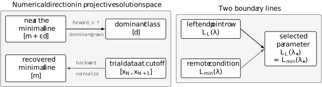
Recurrence direction is projective. Forward evolution magnifies a dominant contaminant; a converged backward sweep recovers the minimal line. A two-endpoint condition requires the independently selected left and remote lines to coincide.

If $\ell$ spans the left line and $m$ spans the remote minimal line, their coincidence can be written

$$\mathcal K_n[\ell,m]=0.$$

Casoratian transport makes this condition independent of the chosen interior index. This is the recurrence analogue of a vanishing boundary Wronskian. The next page turns the equality of the two lines into a continued-fraction condition; later pages connect it to endpoint amplitudes, Green functions, and spectra.

A reproducible recurrence audit

A stable computation should expose its projective and numerical choices:

1. Declare the recurrence sign convention, index origin, parameter tuple, and every exceptional index.
2. Separate a singular endpoint row from the invertible interior recurrence.
3. State which tail is intended and what evidence establishes its minimality.
4. Run backward sweeps over a cutoff sequence $N,N+\Delta,\ldots$.
5. Rescale state pairs during propagation and use a declared nonzero normalization functional.
6. Compare successive cutoffs over the entire required index window, not only at the normalization index.
7. Repeat at higher precision and, when possible, with a different terminal seed or independent representation.
8. Check the recurrence residual and Casoratian transport, while remembering that neither identifies the selected branch.

For a computed sequence $\widehat u$, a scale-aware row residual is

$$\eta_n = \frac{ \left| \alpha_n\widehat u_{n+1} +\beta_n\widehat u_n +\gamma_n\widehat u_{n-1} \right| }{ |\alpha_n\widehat u_{n+1}| +|\beta_n\widehat u_n| +|\gamma_n\widehat u_{n-1}| }.$$

When the denominator vanishes, report the unscaled row separately rather than assigning a misleading relative residual.

Diagnostic	What it tests	What it does not prove
Small $\eta_n$	Algebraic satisfaction of recurrence rows	Correct minimal or dominant branch
Casoratian transport	Indexing, signs, and linear independence	Endpoint admissibility
Cutoff plateau	Stability on the tested finite window	Convergence at an infinite endpoint
Precision plateau	Control of observed roundoff	A theorem for untested parameters

Scope of the next two pages

This page derived the geometry and the finite-cutoff mechanism from an already separated pair. The next page gives coefficient hypotheses, Perron–Kreuser conclusions, Pincherle’s theorem, and continued fractions. The following page develops large-order recurrence asymptotics and estimates the separation ratio that controls cutoff error and connection amplitudes.

Common pitfalls

Calling the smaller displayed value “minimal.” Minimality is an asymptotic ratio between independent solutions. A finite table can suggest a branch but cannot define it.

Treating the dominant solution as unique. The minimal line is unique when it exists. Every $d+c\,m$ belongs to the same dominant asymptotic class, so a dominant normalization must be declared separately.

Assuming a minimal line always exists. Equal-modulus oscillatory solutions can prevent asymptotic separation. Check the hypotheses before invoking backward selection.

Confusing index direction with physical direction. Increasing $n$ is motion in coefficient space, not motion in $z$ or $r$. The relation between coefficient minimality and a physical endpoint requires a convergence argument for the chosen basis.

Starting backward recurrence without normalization. Trial terminal data recover a line, not an absolute solution. A missing or ill-conditioned normalizing functional leaves the answer arbitrary.

Dividing through an exceptional coefficient. A zero of $\alpha_n$ or $\gamma_n$ can signal termination, decoupling, resonance, or a bad parameterization. It is not an invitation to divide by zero and continue.

Using a scalar ratio through a zero. $R_n=u_n/u_{n-1}$ is one projective chart. Switch to the reciprocal ratio or propagate a scaled state vector when its denominator is small.

Trusting the recurrence residual as a branch test. A dominant contaminant is itself a solution. Residuals test the equation, while cutoff and independent-boundary checks test the selected solution.

Equating minimality with endpoint convergence. A minimal coefficient sequence need not make a basis series converge at its boundary without estimates for the basis functions. That bridge is representation-specific.

Exercises

1. Derive the discrete Abel identity

Starting from the house recurrence, derive the Casoratian transport law and its finite-product form.

Solution

Solve both recurrences for the forward entries:

$$\begin{aligned} u_{n+1} &= -\frac{\beta_n}{\alpha_n}u_n -\frac{\gamma_n}{\alpha_n}u_{n-1},\\ v_{n+1} &= -\frac{\beta_n}{\alpha_n}v_n -\frac{\gamma_n}{\alpha_n}v_{n-1}. \end{aligned}$$

Substitution into $\mathcal K_n=u_nv_{n+1}-u_{n+1}v_n$ cancels the two $\beta_n$ terms and leaves

$$\mathcal K_n = \frac{\gamma_n}{\alpha_n} \left( u_{n-1}v_n-u_nv_{n-1} \right) = \frac{\gamma_n}{\alpha_n}\mathcal K_{n-1}.$$

Iteration from $n_0$ to $n$ gives

$$\mathcal K_n = \mathcal K_{n_0} \prod_{j=n_0+1}^{n} \frac{\gamma_j}{\alpha_j}.$$

2. Recover coefficients by Casoratians

If $u=A\,m+B\,d$, prove the two discrete Cramer formulas and explain why they are index-independent.

Solution

Bilinearity and antisymmetry give

$$\begin{aligned} \mathcal K_n[u,d] &= A\mathcal K_n[m,d],\\ \mathcal K_n[m,u] &= B\mathcal K_n[m,d]. \end{aligned}$$

Division by the nonzero basis Casoratian gives $A$ and $B$. Every Casoratian in either ratio is multiplied by the same $\gamma_n/\alpha_n$ when the index advances, so the ratios are constant.

3. Locate the forward instability

For $u_{n+1}-3u_n+2u_{n-1}=0$, derive the perturbed sequence and classify the two fixed points of its forward ratio map.

Solution

The general solution is

$$u_n=A+B2^n.$$

The data $u_0=1$, $u_1=1+\varepsilon$ give $B=\varepsilon$ and $A=1-\varepsilon$, hence

$$u_n=1+\varepsilon(2^n-1).$$

For $R_{n+1}=3-2/R_n$, a fixed point obeys $R^2-3R+2=0$, so $R=1,2$. The derivative $2/R^2$ has magnitudes $2$ and $1/2$, respectively. Thus the minimal fixed point is forward-repelling and the dominant fixed point is forward-attracting.

4. Prove the finite-cutoff formula

Assume $m_n/d_n\to0$, impose $x_{N+1}=0$, and normalize at an anchor $k$ with $m_k\neq0$ and $m_k-r_Nd_k\neq0$. Derive the displayed formula for $\widehat x_n^{(N)}$ and its exact cutoff error.

Solution

Write $x=A_Nm+B_Nd$. The terminal condition gives

$$B_N/A_N=-m_{N+1}/d_{N+1}=-r_N.$$

The value of $x_N$ fixes only the common scale. Division by the value at $k$ yields

$$\widehat x_n^{(N)} = \frac{m_n-r_Nd_n}{m_k-r_Nd_k}.$$

Subtracting $m_n/m_k$ over a common denominator gives

$$\widehat x_n^{(N)} -\frac{m_n}{m_k} = \frac{ r_N(m_nd_k-m_kd_n) }{ m_k(m_k-r_Nd_k) }.$$

For fixed $n,k$, the right-hand side tends to zero with $r_N$, provided $m_k\neq0$ and the finite-cutoff normalization denominator stays away from zero.

5. Compare exponential and polynomial separation

Verify the solutions $m_n=1/(n+1)$ and $d_n=1$ of the variable-coefficient example. Derive its normalized backward cutoff error.

Solution

For $m$ the three recurrence terms reduce to

$$1-2+1=0,$$

and the same cancellation is immediate for $d=1$. Solving the terminal conditions in $x_n=A/(n+1)+B$ gives

$$\begin{aligned} A&=(N+1)(N+2),\\ B&=-(N+1). \end{aligned}$$

Therefore

$$x_n^{(N)} = \frac{(N+1)(N+1-n)}{n+1}.$$

Since $x_0^{(N)}=(N+1)^2$,

$$\widehat x_n^{(N)} = \frac1{n+1} \left( 1-\frac{n}{N+1} \right),$$

and division by $m_n$ gives relative error $-n/(N+1)$.

6. Exhibit a recurrence with no minimal solution

Show that no nonzero solution of $u_{n+1}-u_{n-1}=0$ is minimal at $+\infty$.

Solution

Every solution has the form

$$u_n=A+B(-1)^n.$$

Let an independent comparison solution be $g_n=C+D(-1)^n$. If it is nonzero eventually, then $C+D$ and $C-D$ are both nonzero. The condition $u_n/g_n\to0$ along the even and odd subsequences would force $A+B=0$ and $A-B=0$, hence $u=0$. If one of $C\pm D$ vanishes, $g$ has infinitely many zero entries and is not an admissible eventual denominator for the scalar-ratio definition. Thus no nonzero solution is minimal. The characteristic roots $1$ and $-1$ have equal modulus, so neither projective direction separates.

7. Interpret the Leaver endpoint rows

Explain why $a_{-1}=0$ together with the $n=0$ recurrence row selects a line but neither an absolute normalization nor the remote boundary condition.

Solution

The first row is

$$\mathsf A_0a_1+\mathsf B_0a_0=0.$$

When $\mathsf A_0\neq0$, it fixes the ratio $a_1/a_0=-\mathsf B_0/\mathsf A_0$. Multiplying every $a_n$ by the same constant preserves the recurrence, so an additional convention such as $a_0=1$ is required for absolute normalization.

The first row contains no information about the $n\to\infty$ tail. A remote condition supplies a second projective line, often the minimal line. Both conditions hold only when the two lines coincide; equivalently, their Casoratian vanishes.

References

• NIST Digital Library of Mathematical Functions, §3.6, Linear Difference Equations, especially the homogeneous-equation discussion, Miller’s algorithm, normalization, cutoff comparison, and the Bessel example.
• NIST Digital Library of Mathematical Functions, §2.9, Difference Equations, for the asymptotic theory developed on the next pages.
• W. Gautschi, “Computational Aspects of Three-Term Recurrence Relations,” SIAM Review 9 (1967), 24–82, DOI: 10.1137/1009002.
• F. W. J. Olver, “Error Analysis of Miller’s Recurrence Algorithm,” Mathematics of Computation 18 (1964), 65–74, DOI: 10.2307/2003406.
• F. W. J. Olver, “Numerical Solution of Second-Order Linear Difference Equations,” Journal of Research of the National Bureau of Standards B 71B (1967), 111–129, DOI: 10.6028/jres.071B.018.
• A. Gil, J. Segura, and N. M. Temme, Numerical Methods for Special Functions, Chapter 4, SIAM, 2007, DOI: 10.1137/1.9780898717822.ch4.
• J. Wimp, Computation with Recurrence Relations, Pitman, 1984, ISBN 978-0-273-08508-9.