Large-Order Recurrence Asymptotics and Connection Amplitudes

Pincherle’s theorem identifies a line at infinity. Large-order asymptotics put a scale on that line, quantify its separation from the competing line, and provide useful terminal data for a backward sweep. Neither operation, by itself, fixes an absolute connection amplitude.

The central chain on this page is

$$\begin{gathered} \text{ratio expansion}\\ \Downarrow\\ \text{coefficient scale}\\ \Downarrow\\ \text{minimal/dominant basis}\\ \Downarrow\\ \text{normalized connection amplitude}\\ \Downarrow\\ \text{ODE endpoint coefficient}. \end{gathered}$$

Every arrow has hypotheses. In particular, substituting a formal series into a recurrence is not an existence proof, and a coefficient amplitude is not automatically a physical wave amplitude.

A status firewall for asymptotic claims

Several mathematically different statements are often compressed into the phrase “the large-$n$ solution.” Keep them separate:

Claim	Status and required evidence
A balance predicts a ratio scale	Formal Newton or dominant-balance calculation
Coefficient comparison produces a series	Formal identity to the computed order
Exact solutions possess those expansions	Asymptotic-existence theorem with its hypotheses checked
A remainder is smaller than the last term	Remainder theorem, not formal substitution alone
A finite-depth answer is stable	Numerical observation over depth and precision
A coefficient is a physical amplitude	Basis normalization and a valid series-to-endpoint transfer

The Wong–Li theorems invoked below construct exact solutions for fixed recurrence parameters in the regular distinct-root and generic double-root cases. They do not automatically provide parameter-uniform analyticity near a root collision, a transition ray, or a finite singularity of the recurrence.

Ratios integrate into factorial and exponential scales

For the house recurrence

$$\alpha_nu_{n+1} +\beta_nu_n +\gamma_nu_{n-1} =0,$$

write

$$R_n=\frac{u_n}{u_{n-1}}.$$

Then

$$u_n=u_0\prod_{k=1}^{n}R_k.$$

This elementary product is the bridge from ratio asymptotics to sequence asymptotics. If, formally,

$$R_n \sim \lambda n^\eta \left( 1+\sum_{j\geq1}d_jn^{-j/p_*} \right),$$

where $p_*\in\mathbb N$ is the Puiseux denominator. Expand the logarithm as

$$\log\left( 1+\sum_{j\geq1}d_jx^j \right) = \sum_{j\geq1}\ell_jx^j.$$

Euler–Maclaurin summation then gives the scale

$$\begin{aligned} u_n\sim{}& C\lambda^n\Gamma(n+1)^\eta\\ &\times \exp\left[ \sum_{j=1}^{p_*-1} \frac{\ell_j}{ 1-j/p_* } n^{1-j/p_*} \right] n^{\ell_{p_*}} \left(1+\cdots\right). \end{aligned}$$

This formula is best read as a dictionary:

• $\lambda$ produces an ordinary geometric factor $\lambda^n$;
• $n^\eta$ in the ratio produces $\Gamma(n+1)^\eta$;
• a ratio correction $n^{-\delta}$ with $0<\delta<1$ produces a stretched exponential $\exp(cn^{1-\delta})$;
• the $n^{-1}$ term in the logarithm of the ratio produces an algebraic power of $n$.

The last point prevents a common error. If

$$R_n^\pm = r\left[ 1\pm\kappa n^{-1/2} +c_2n^{-1} +O(n^{-3/2}) \right],$$

then

$$\log\frac{R_n^\pm}{r} = \pm\kappa n^{-1/2} +\left( c_2-\frac{\kappa^2}{2} \right)n^{-1} +O(n^{-3/2}),$$

and hence

$$u_n^\pm \sim C_\pm r^n \exp\left(\pm2\kappa\sqrt n\right) n^{\,c_2-\kappa^2/2} \left[ 1+O(n^{-1/2}) \right].$$

The power is $c_2-\kappa^2/2$, not $c_2$.

Exact asymptotic solutions for regular tails

Put a regular tail into the standard form

$$w(n+2)+f(n)w(n+1)+g(n)w(n)=0,$$

where

$$\begin{aligned} f(n)&\sim\sum_{s\geq0}f_sn^{-s},\\ g(n)&\sim\sum_{s\geq0}g_sn^{-s}, & g_0&\neq0. \end{aligned}$$

The expansions here are Poincaré asymptotic expansions with the remainder conditions required by the theorem being invoked.

For the two cases used below, the operational checklist is:

• hold the recurrence parameters fixed;
• require $f$ and $g$ to possess the stated coefficient expansions with remainders through every order used;
• require $g_0\neq0$ and an eventually nonsingular recurrence tail;
• impose either two distinct characteristic roots, as in DLMF §2.9(i), or a double root with nonzero square-root splitting, as in DLMF §2.9(ii).

Wong and Li prove the existence statements behind those two DLMF cases. Checking this list at one parameter does not establish locally uniform control as the parameter varies.

Distinct characteristic roots

Let $r_1,r_2$ be the distinct roots of

$$P(r)=r^2+f_0r+g_0.$$

Under the Wong–Li hypotheses, there are independent exact solutions

$$w_j(n) \sim r_j^n n^{\alpha_j} \sum_{s=0}^{\infty} \frac{a_{s,j}}{n^s}, \qquad a_{0,j}=1,$$

where

$$\alpha_j = \frac{f_1r_j+g_1}{ f_0r_j+2g_0 } = -\frac{f_1r_j+g_1}{ r_jP'(r_j) }.$$

The preceding page used unequal root moduli to select a minimal branch. The refined form reveals another possibility. If $|r_1|=|r_2|$ but

$$\operatorname{Re}\alpha_1 < \operatorname{Re}\alpha_2,$$

then $w_1/w_2\to0$ algebraically, so $w_1$ is still minimal. If both the root moduli and the real algebraic exponents agree, this level of asymptotics is inconclusive.

A generic repeated root

Now suppose

$$P(r)=(r-r_0)^2, \qquad r_0\neq0.$$

Thus $f_0=-2r_0$ and $g_0=r_0^2$. Define

$$\kappa^2 = -\frac{f_1r_0+g_1}{r_0^2}.$$

If $\kappa\neq0$, the generic coincident-root theorem supplies exact solutions of the form

$$w_\pm(n) \sim r_0^n \exp\left(\pm2\kappa\sqrt n\right) n^\alpha \sum_{s=0}^{\infty} c_s^{(\pm)}n^{-s/2},$$

with

$$c_0^{(+)}=c_0^{(-)}=1$$

and

$$\alpha = \frac{g_0+2g_1}{4g_0}.$$

Equivalently, the stretched-exponential coefficient used in DLMF §2.9 is $2\kappa$, and

$$(2\kappa)^2 = \frac{2f_0f_1-4g_1}{g_0}.$$

Choose a square-root branch continuously on the parameter domain. If $\operatorname{Re}\kappa>0$, the minus solution is minimal and

$$\frac{w_-(n)}{w_+(n)} \sim \exp\left(-4\kappa\sqrt n\right).$$

If $\operatorname{Re}\kappa=0$, the two displayed envelopes have equal modulus on the positive-index ray; this leading expansion does not order them. If $\kappa=0$, the half-integer ansatz itself degenerates.

The degenerate double-root case

When $2g_1=f_0f_1$, do not set $\kappa=0$ in the generic formula and keep going. The algebraic indices must instead be found from

$$\begin{aligned} 2g_0\alpha^2 &-\left(f_0f_1+2g_0\right)\alpha\\ &+2g_2-f_0f_2=0. \end{aligned}$$

If the two indices coincide, the second independent solution has a logarithmic companion. A nonzero integral difference permits a logarithm, but its coefficient may vanish. This is a difference-equation analogue of Frobenius resonance.

The repeated-root calculation in ratio form

The practical calculation can be done without first guessing the full sequence. After multiplication of a recurrence row by a harmless common factor, suppose

$$\begin{aligned} \alpha_n &= n^2\left( 1+\frac{A_1}{n} +\frac{A_2}{n^2} +\cdots \right),\\ \beta_n &= n^2\left( -2+\frac{B_1}{n} +\frac{B_2}{n^2} +\cdots \right),\\ \gamma_n &= n^2\left( 1+\frac{C_1}{n} +\frac{C_2}{n^2} +\cdots \right). \end{aligned}$$

The limiting polynomial is $(r-1)^2$. Dividing the $n$th row by $u_n$ gives the exact Riccati equation

$$\alpha_nR_{n+1} +\beta_n +\frac{\gamma_n}{R_n} =0.$$

Insert

$$R_n^{(\varepsilon)} = 1+\varepsilon\kappa n^{-1/2} +r_1n^{-1} +O(n^{-3/2}), \qquad \varepsilon\in\{+1,-1\}.$$

The first two nontrivial coefficient equations are

$$\kappa^2+A_1+B_1+C_1=0$$

and

$$2r_1 = \kappa^2-A_1+C_1+\frac12.$$

Therefore

$$\begin{aligned} \kappa^2 &= -\left(A_1+B_1+C_1\right),\\ r_1 &= \frac12\left( \kappa^2-A_1+C_1+\frac12 \right),\\ p &= r_1-\frac{\kappa^2}{2} = \frac{C_1-A_1}{2}+\frac14. \end{aligned}$$

The corresponding formal sequence scales are

$$u_n^{(\varepsilon)} \sim C_\varepsilon \exp\left( 2\varepsilon\kappa\sqrt n \right) n^p \left[ 1+O(n^{-1/2}) \right].$$

The nonzero constants $C_\varepsilon$ are arbitrary normalizations; the ratio calculation cannot determine them.

This coefficient comparison is a convenient derivation engine. The existence theorem in the preceding section is what promotes the formal scales to asymptotic expansions of exact solutions.

Schwarzschild coefficients split on the square-root scale

Return to the Jaffé–Leaver recurrence derived earlier:

$$\mathsf A_na_{n+1} +\mathsf B_na_n +\mathsf C_na_{n-1} =0,$$

where

$$\mathsf A_n=(n+1)(n+2\varrho+1),$$ $$\begin{aligned} \mathsf B_n =-\bigl[ &2n^2+(8\varrho+2)n\\ &+8\varrho^2+4\varrho +\ell(\ell+1)-\sigma \bigr], \end{aligned}$$

and

$$\mathsf C_n=(n+2\varrho)^2-s^2.$$

The physical specialization used here is

$$\sigma=s^2-1.$$

Dividing the three coefficients by $n^2$ gives

$$\begin{aligned} A_1&=2\varrho+2,\\ B_1&=-8\varrho-2,\\ C_1&=4\varrho. \end{aligned}$$

Consequently,

$$\kappa^2=2\varrho, \qquad p=\varrho-\frac34.$$

On a domain where $\varrho\neq0$, choose

$$\kappa=\sqrt{2\varrho}$$

continuously. If $\operatorname{Re}\kappa>0$, the exact minimal and dominant tails may be normalized so that

$$\begin{aligned} m_n &\sim n^{\varrho-3/4} \exp\left(-2\kappa\sqrt n\right) \left[ 1+O(n^{-1/2}) \right],\\ d_n &\sim n^{\varrho-3/4} \exp\left(+2\kappa\sqrt n\right) \left[ 1+O(n^{-1/2}) \right]. \end{aligned}$$

Thus

$$\frac{m_n}{d_n} = O\left( \exp\left[-4\operatorname{Re}(\kappa)\sqrt n\right] \right).$$

This is the missing tail theorem behind the continued-fraction candidate on the preceding page.

Four terms of the Schwarzschild ratio

Let

$$R_n=\frac{a_n}{a_{n-1}}, \qquad L=\ell(\ell+1).$$

Substitution into

$$\mathsf A_nR_{n+1}R_n +\mathsf B_nR_n +\mathsf C_n=0$$

gives

$$\begin{aligned} R_n^{(\varepsilon)} ={}& 1+\varepsilon\kappa n^{-1/2} +\left(2\varrho-\frac34\right)n^{-1}\\ &+\varepsilon c_3n^{-3/2} +c_4n^{-2} +O(n^{-5/2}), \end{aligned}$$

where

$$c_3 = \frac{ 64\varrho^2-48\varrho+16L+3 }{ 32\kappa }$$

and

$$c_4 = \frac{ 64\varrho(L-s^2)+48\varrho+16L+3 }{ 128\varrho }.$$

The spin cancels through $c_3$ and first appears in $c_4$. This cancellation uses $\sigma=s^2-1$; it should not be imposed while deriving a recurrence for a different equation.

Taking logarithms and choosing unit leading normalization reproduces

$$a_n^{(\varepsilon)} \sim n^{\varrho-3/4} \exp\left( 2\varepsilon\kappa\sqrt n \right) \left[ 1+O(n^{-1/2}) \right].$$

At $\varrho=0$, the displayed coefficients are nonuniform. The ratio then has an algebraic form $R_n=1+\chi/n+\cdots$, with

$$\chi^2+\chi+1-L+\sigma-s^2=0.$$

For $\sigma=s^2-1$, the indices are $\chi=\ell$ and $\chi=-\ell-1$. The square-root seed must not be used near this transition unless the depth is large compared with the nonuniform scale $|\kappa|^{-2}$.

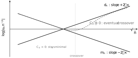
Repeated-root splitting on the $\sqrt n$ scale. After removal of the common power $n^p$, the minimal and dominant envelopes have slopes $-2\operatorname{Re}\kappa$ and $+2\operatorname{Re}\kappa$. A mixture $C_mm+C_dd$ eventually follows the dominant line whenever $C_d\neq0$.

Ignoring lower-order corrections, the crossover occurs near

$$\sqrt{n_{\mathrm{cross}}} \approx \frac{ \log\lvert C_m/C_d\rvert }{ 4\operatorname{Re}\kappa },$$

when the right-hand side is positive. A tiny unwanted amplitude can therefore remain hidden for a long finite range.

For $\operatorname{Re}\kappa>0$, the minimal coefficients obey

$$\sum_{n\geq0}n^j\lvert m_n\rvert<\infty$$

for every fixed nonnegative integer $j$. Hence the minimal Jaffé power series factor and every fixed termwise $x$-derivative of that factor converge absolutely at $x=1$. This does not imply analytic continuation through $x=1$, nor does it bypass differentiation of the prefactor and $x(r)$ when derivatives of the full ODE solution are needed.

Asymptotic tail seeds and cutoff separation

A backward ratio sweep ending at row $N$ requires a terminal value for $R_{N+1}$. The zero tail

$$R_{N+1}=0$$

is valid as a projective cutoff but discards known large-order information. For the Schwarzschild minimal branch, a four-term asymptotic seed is

$$\begin{aligned} R_{N+1}^{\mathrm{seed}} ={}& 1-\frac{\kappa}{\sqrt{N+1}} +\frac{2\varrho-\frac34}{N+1}\\ &-\frac{c_3}{(N+1)^{3/2}} +\frac{c_4}{(N+1)^2}. \end{aligned}$$

The index $N+1$ matters: $R_n=a_n/a_{n-1}$. A formula for $a_{n+1}/a_n$ is shifted by one row.

There is an exact way to see what a terminal seed controls. Let $m,d$ be an exact minimal–dominant basis and let a trial solution be

$$x=m+\lambda d.$$

If its terminal ratio is

$$T_N=\frac{x_{N+1}}{x_N},$$

then

$$\lambda = \frac{m_N}{d_N} \frac{ R_{N+1}^{m}-T_N }{ T_N-R_{N+1}^{d} }.$$

For a zero tail this becomes

$$\lambda = -\frac{m_{N+1}}{d_{N+1}} = O\left( \exp\left[-4\operatorname{Re}(\kappa)\sqrt N\right] \right).$$

An asymptotic seed makes the numerator $R_{N+1}^{m}-T_N$ smaller. Turning its formal omitted term into a rigorous head-error bound additionally requires a remainder estimate and control of the denominator. A small substituted Riccati defect alone is not such a bound.

A reproducible finite-depth benchmark

At the algebraic test point

$$\varrho=\frac14, \qquad \ell=2, \qquad s=2, \qquad \sigma=3,$$

the minimal ratio is

$$\begin{aligned} R_n^{\min} ={}& 1-\frac{1}{\sqrt{2n}} -\frac{1}{4n} -\frac{91\sqrt2}{32n^{3/2}}\\ &+\frac{143}{32n^2} +O(n^{-5/2}). \end{aligned}$$

The reference uses 100-decimal-digit arithmetic, cutoff $N_{\mathrm{ref}}=10\,000$, and the displayed $n^{-2}$ seed evaluated at $R_{10\,001}$. The backward map is applied down to $R_1$. Doubling the cutoff to $20\,000$ and raising the working precision to 150 digits leaves all digits quoted below unchanged:

$$\begin{aligned} R_1^{\min} = -0.1776779698080973454908003349989862\ldots. \end{aligned}$$

Every finite-depth sweep in the following table was also performed at 100-digit working precision and compared with that same reference. The absolute errors in $R_1$ are:

$N$	Zero tail	Seed through $n^{-3/2}$	Seed through $n^{-2}$
$10$	$1.4392\times10^{-6}$	$1.9993\times10^{-7}$	$4.9958\times10^{-8}$
$20$	$1.3612\times10^{-8}$	$6.7614\times10^{-10}$	$1.6424\times10^{-10}$
$40$	$3.2221\times10^{-11}$	$5.5849\times10^{-13}$	$1.2359\times10^{-13}$
$80$	$1.0388\times10^{-14}$	$6.1343\times10^{-17}$	$1.1711\times10^{-17}$

These are numerical observations, not certified bounds. They do, however, audit the indexing and signs: successive half-orders improve the same backward limit, while the zero tail converges on the predicted stretched-exponential scale. The reporting rule is conservative: retain only digits unchanged when both the cutoff is doubled and the working precision is increased.

The idea is often called a Nollert improvement in quasinormal-mode calculations. It is more general: any recurrence with a controlled large-order ratio expansion can use the expansion as terminal projective data.

Recurrence connection amplitudes from Casoratians

Ratios are invariant under $u\mapsto cu$, so they cannot determine an absolute amplitude. First normalize exact tail solutions by specified unit-leading asymptotic models:

$$\frac{m_n}{\mathfrak m_n}\longrightarrow1, \qquad \frac{d_n}{\mathfrak d_n}\longrightarrow1.$$

To avoid collision with the angular index $\ell$, denote a left-normalized solution by $u^{\mathrm L}$ and write

$$u^{\mathrm L}=C_mm+C_dd.$$

With the chapter convention

$$\mathcal K_n[u,v] = u_nv_{n+1}-u_{n+1}v_n,$$

the exact coordinates are

$$\begin{aligned} C_m &= \frac{ \mathcal K_n[u^{\mathrm L},d] }{ \mathcal K_n[m,d] },\\ C_d &= \frac{ \mathcal K_n[m,u^{\mathrm L}] }{ \mathcal K_n[m,d] }. \end{aligned}$$

Both quotients are independent of $n$: numerator and denominator obey the same discrete Abel scaling. Since $m_n/d_n\to0$,

$$C_d = \lim_{n\to\infty} \frac{u_n^{\mathrm L}}{d_n} = \lim_{n\to\infty} \frac{u_n^{\mathrm L}}{\mathfrak d_n}.$$

This limit is useful for measuring a dominant amplitude. It is a poor way to recover $C_m$ from a generic mixture, because forward arithmetic erases the subdominant part.

The normalization ledger

The amplitude changes with the normalization of the objects it compares:

$$u^{\mathrm L}\mapsto q\,u^{\mathrm L}, \qquad d\mapsto td \quad\Longrightarrow\quad \begin{aligned} C_m&\mapsto qC_m,\\ C_d&\mapsto\frac{q}{t}C_d. \end{aligned}$$

There is a subtler ambiguity. The replacement

$$d\mapsto d+c\,m$$

does not change the complete dominant Poincaré expansion, because $m$ is beyond all algebraic orders relative to $d$. It leaves $C_d$ invariant but changes

$$C_m\mapsto C_m-cC_d.$$

Thus the unwanted dominant amplitude is canonical after the left and dominant leading normalizations are fixed. A full pair of exact connection coefficients needs an additional analytic prescription for the dominant complement.

The continued-fraction residual and the unwanted amplitude

Normalize the left solution by

$$u_0^{\mathrm L}=1, \qquad u_1^{\mathrm L}=-\frac{\beta_0}{\alpha_0},$$

and let $m$ be the exact minimal solution. The Leaver residual is

$$F_0 = \beta_0+\alpha_0\frac{m_1}{m_0}.$$

At the first row,

$$\mathcal K_0[m,u^{\mathrm L}] = m_0u_1^{\mathrm L}-m_1u_0^{\mathrm L} = -\frac{m_0}{\alpha_0}F_0.$$

Therefore the dominant recurrence amplitude is

$$C_d = -\frac{m_0}{ \alpha_0\mathcal K_0[m,d] } F_0.$$

The residual and $C_d$ have the same zeros wherever the displayed prefactor is finite and nonzero, but they are not the same normalized function. At a ratio-chart pole, use homogeneous pairs and Casoratians rather than this affine formula.

If the series-to-ODE map is denoted by $\mathscr S$ and the endpoint ODE basis is unit-normalized as

$$\mathscr S[m]=\nu_m y_{\mathrm{adm}}, \qquad \mathscr S[d]=\nu_d y_{\mathrm{bad}},$$

then

$$\mathscr S[u^{\mathrm L}] = \nu_mC_m y_{\mathrm{adm}} +\nu_dC_d y_{\mathrm{bad}}.$$

The physical bad-endpoint coefficient is $\nu_dC_d$, not automatically $C_d$ and not automatically $F_0$.

Darboux transfer for algebraic endpoint amplitudes

Coefficient tails can encode endpoint connection coefficients directly. Assume in this subsection that

$$\mu\notin\{0,-1,-2,\ldots\}.$$

The excluded values are polynomial or limiting cases and do not obey the coefficient-limit formula below without separate treatment. The exact binomial identity

$$(1-x)^{-\mu} = \sum_{n=0}^{\infty} \frac{ \Gamma(n+\mu) }{ \Gamma(\mu)\Gamma(n+1) } x^n$$

implies

$$[x^n](1-x)^{-\mu} \sim \frac{n^{\mu-1}}{\Gamma(\mu)}.$$

More generally, suppose $F$ has the required continuation to a $\Delta$-domain at $x=1$, no competing boundary singularity contributes at the same scale, and

$$F(x) \sim A(1-x)^{-\mu}.$$

Then the transfer theorem gives

$$[x^n]F(x) \sim \frac{A}{\Gamma(\mu)}n^{\mu-1},$$

so

$$A = \Gamma(\mu) \lim_{n\to\infty} n^{1-\mu}[x^n]F(x).$$

This direction is a theorem under the stated analyticity hypotheses. The converse is not automatic: the same coefficient asymptotics need not, by itself, prove a unique local singular expansion.

An exact hypergeometric audit

Let

$$F(x)={}_2F_1(a,b;c;x) = \sum_{n=0}^{\infty}u_nx^n,$$

with

$$u_n = \frac{(a)_n(b)_n}{(c)_n\,n!}.$$

Put $\mu=a+b-c$ and assume

$$\begin{gathered} c\notin\mathbb Z_{\leq0}, \qquad a,b\notin\mathbb Z_{\leq0},\\ \mu\notin\mathbb Z. \end{gathered}$$

These conditions exclude denominator poles, terminating numerator series, and the resonant connection cases. Gamma-ratio asymptotics give

$$u_n \sim \frac{\Gamma(c)}{ \Gamma(a)\Gamma(b) } n^{\mu-1}.$$

The unit-leading singular solution at $x=1$ begins with $(1-x)^{-\mu}$, and its exact connection coefficient is

$$B = \frac{ \Gamma(c)\Gamma(\mu) }{ \Gamma(a)\Gamma(b) }.$$

Darboux transfer recovers the same entry:

$$B = \Gamma(\mu) \lim_{n\to\infty} n^{1-\mu}u_n.$$

For

$$a=\frac12, \qquad b=\frac23, \qquad c=1,$$

one has $\mu=1/6$ and

$$B = \frac{ \Gamma(1/6) }{ \sqrt\pi\,\Gamma(2/3) } \approx 2.3191905339278567.$$

This independently checks the power, the gamma factor, and the unit-leading endpoint normalization against the connection matrix derived in Chapter 2.

A finite-order amplitude estimator

For the exact test function

$$F(x) = \frac75(1-x)^{-3/2} = \sum_{n=0}^{\infty}a_nx^n,$$

define

$$\widehat A_n = \Gamma(3/2)a_n n^{-1/2}.$$

Then $\widehat A_n\to7/5$. Since

$$\widehat A_n = \frac75 \left( 1+\frac{3}{8n} +O(n^{-2}) \right),$$

division by $1+3/(8n)$ removes the first correction:

$n$	Raw $\widehat A_n$	First-correction estimate
$5$	$1.5020391188$	$1.3972456919$
$10$	$1.4517469054$	$1.3992741257$
$50$	$1.4104694738$	$1.3999697011$
$200$	$1.4026230875$	$1.3999980911$

An extrapolated coefficient is still conditional on the assumed transfer model. Several singularities on the same convergence circle contribute a sum of asymptotic terms and must be separated before applying this one-singularity estimator.

The Schwarzschild endpoint amplitude

For the Jaffé representation used earlier,

$$\begin{aligned} \psi(r) ={}& (r-1)^\varrho r^{-2\varrho} \exp[-\varrho(r-1)]\\ &\times \sum_{n=0}^{\infty} a_n \left( \frac{r-1}{r} \right)^n. \end{aligned}$$

Put

$$x=\frac{r-1}{r}, \qquad S(x)=\sum_{n=0}^{\infty}a_nx^n.$$

At a spectral parameter satisfying $F_0=0$, the left-normalized coefficient sequence is minimal. If $\operatorname{Re}\kappa>0$, then

$$S(1)=\sum_{n=0}^{\infty}a_n$$

converges absolutely. Relative to the unit remote behavior

$$r^{-\varrho}\exp(-\varrho r),$$

the endpoint amplitude is

$$A_{\mathrm{adm}} = \exp(\varrho)S(1).$$

The factor $\exp(\varrho)$ comes from the prefactor; omitting it is a normalization error.

The minimal tail also estimates the endpoint-sum remainder. If

$$a_n \sim C_mn^{\varrho-3/4} \exp(-2\kappa\sqrt n),$$

then, in a sector where the integral comparison is valid,

$$\sum_{n>N}a_n \sim \frac{C_m}{\kappa} N^{\varrho-1/4} \exp(-2\kappa\sqrt N).$$

This provides a useful tail correction after $C_m$ has been fitted or computed by a Casoratian.

The unwanted dominant tail has a different transfer mechanism. For a generic left sequence with

$$a_n \sim C_dn^{\varrho-3/4} \exp(+2\kappa\sqrt n),$$

put $x=\exp(-\tau)$. Assume $\tau\to0$ with $\operatorname{Re}\tau>0$, so $|x|<1$, in a fixed sector for which

$$\left| \arg\frac{\kappa}{\sqrt\tau} \right| < \frac{\pi}{4}-\epsilon$$

with some $\epsilon>0$. For positive real $\tau$, this is $|\arg\kappa|<\pi/4-\epsilon$. In this sector the interior saddle is accessible and dominant. Replacing the tail sum by its continuum model and setting $n=t^2$ gives

$$\begin{aligned} S(\exp[-\tau]) \sim 2C_d\int_0^\infty &t^{2\varrho-1/2}\\ &\times \exp(2\kappa t-\tau t^2)\,\dd t. \end{aligned}$$

The phase has saddle $t_*=\kappa/\tau$. Completing the square supplies $\exp(\kappa^2/\tau)=\exp(2\varrho/\tau)$, while the Gaussian width contributes $\sqrt{\pi/\tau}$. Combining the remaining powers gives, in the corresponding validity sector,

$$\begin{aligned} S(x) \sim{}& 2\sqrt\pi\,C_d \kappa^{\,2\varrho-1/2}\\ &\times \tau^{-2\varrho} \exp\left(\frac{2\varrho}{\tau}\right). \end{aligned}$$

Since $\tau^{-1}=r-\tfrac12+O(r^{-1})$, multiplication by the Jaffé prefactor produces the opposite remote wave $r^\varrho\exp(\varrho r)$ with coefficient

$$B_{\mathrm{opp}} = 2\sqrt\pi\,C_d \kappa^{\,2\varrho-1/2}.$$

Thus the dominant coefficient-tail amplitude is proportional to the unwanted physical connection amplitude, with a calculable normalization. The power of $\kappa$ uses the branch induced by its declared continuous choice. Outside the stated saddle sector, analytic continuation and Stokes control are required; the coefficient tail alone does not justify retaining an exponentially subdominant saddle contribution. At a quasinormal-mode zero, $C_d=0$; the minimal sum instead yields $A_{\mathrm{adm}}$.

A numerical workflow that preserves the mathematics

1. Record the original recurrence, row scaling, exceptional indices, parameter point, and square-root branch.
2. Derive the ratio expansion in the original indexing and substitute it back to record its formal defect order.
3. Check the hypotheses of an asymptotic-existence theorem before calling the formal branches exact minimal and dominant solutions.
4. Evaluate the minimal seed at the actual terminal ratio index $N+1$.
5. Sweep backward with homogeneous pairs and rescale them, switching ratio charts near poles.
6. Compare zero-tail and successive asymptotic seeds over several depths and precisions. Treat agreement as evidence unless an error theorem supplies constants.
7. Measure zeros with the homogeneous Casoratian or residual; measure an absolute amplitude only after fixing both basis normalizations.
8. Translate the recurrence amplitude to an ODE amplitude with the representation factor, then audit it against direct ODE matching or an exact special-function benchmark.

Near $\operatorname{Re}\kappa=0$ or $\kappa=0$, fixed-parameter tail asymptotics are nonuniform. Increasing precision cannot compensate for a depth that is too short to resolve the branch separation.

Handoff to the next page

This page treats nonterminating tails and their asymptotic normalization. The next page distinguishes those cutoffs from exact polynomial termination, then develops finite and Hill determinants and their quasi-exact sectors.

Common pitfalls

Promoting a formal balance to a theorem. Coefficient comparison proves that a series formally cancels the recurrence. An asymptotic-existence theorem is what supplies exact solutions having that series.

Changing the square-root branch point by point. The labels “plus” and “minus” are meaningful only after $\sqrt{2\varrho}$ is continued on a declared parameter domain. Crossing a branch cut can exchange the two labels.

Using a repeated-root seed at its transition. The half-power expansion is singular at $\varrho=0$ and loses separation when $\operatorname{Re}\sqrt{2\varrho}=0$. Recompute the relevant algebraic or transition asymptotics.

Inferring an absolute amplitude from ratios. Ratios determine a projective line. A connection amplitude additionally requires normalizations for the left solution and the endpoint basis.

Calling the residual the physical coefficient. $F_0$, $C_d$, and the ODE bad-endpoint coefficient have the same generic zeros but differ by normalization factors.

Extracting a subdominant coefficient by forward subtraction. Once the dominant branch overwhelms a floating-point sequence, subtracting it leaves mostly roundoff. Use a Casoratian, backward propagation, or a matched basis.

Treating a tail seed as an error certificate. A higher-order seed often accelerates convergence dramatically. Certification still requires a remainder bound, denominator control, and a valid depth range.

Applying one-singularity Darboux transfer blindly. Competing singularities on the convergence circle, logarithmic resonance, or a missing continuation domain change the coefficient asymptotics.

Exercises

1. Integrate a half-power ratio

Suppose

$$R_n = r\left( 1+\kappa n^{-1/2} +cn^{-1} +O(n^{-3/2}) \right).$$

Derive the leading asymptotic form of $u_n$.

Solution

Take logarithms:

$$\log R_n = \log r +\kappa n^{-1/2} +\left(c-\frac{\kappa^2}{2}\right)n^{-1} +O(n^{-3/2}).$$

Use

$$\sum_{k=1}^{n}k^{-1/2} = 2\sqrt n+O(1), \qquad \sum_{k=1}^{n}k^{-1} = \log n+O(1).$$

The summable remainder changes only the constant and lower corrections, so

$$u_n \sim Cr^n \exp(2\kappa\sqrt n) n^{c-\kappa^2/2}.$$

2. Derive the repeated-root balance

For the normalized coefficients $A_1,B_1,C_1$ on this page, substitute the half-power ratio ansatz and recover $\kappa^2$, $r_1$, and $p$.

Solution

Expand

$$\begin{aligned} R_{n+1} ={}& 1+\varepsilon\kappa n^{-1/2} +r_1n^{-1}\\ &+\varepsilon \left( r_2-\frac{\kappa}{2} \right)n^{-3/2} +O(n^{-2}). \end{aligned}$$

and

$$\begin{aligned} \frac1{R_n} ={}& 1-\varepsilon\kappa n^{-1/2} +(\kappa^2-r_1)n^{-1}\\ &+\varepsilon \left( -r_2+2\kappa r_1-\kappa^3 \right)n^{-3/2} +O(n^{-2}). \end{aligned}$$

Here $\varepsilon r_2$ denotes the unneeded next coefficient in the ratio ansatz. In

$$\alpha_nR_{n+1} +\beta_n +\frac{\gamma_n}{R_n} =0,$$

the $n^{-1}$ coefficient gives

$$\kappa^2+A_1+B_1+C_1=0.$$

The $r_2$ terms cancel from the $n^{-3/2}$ coefficient, which gives

$$2r_1 = \kappa^2-A_1+C_1+\frac12.$$

Finally $p=r_1-\kappa^2/2$, because the logarithm of the ratio contains $r_1-\kappa^2/2$ at order $n^{-1}$.

3. Resolve the Schwarzschild tail

Use the displayed Schwarzschild coefficients to prove

$$\kappa^2=2\varrho, \qquad p=\varrho-\frac34.$$

At $\varrho=1/4$, show that the minimal series and all of its fixed termwise $x$-derivatives converge absolutely at $x=1$.

Solution

The normalized first coefficients are

$$A_1=2\varrho+2, \quad B_1=-8\varrho-2, \quad C_1=4\varrho.$$

Therefore

$$\kappa^2 = -(A_1+B_1+C_1) = 2\varrho$$

and

$$p = \frac{C_1-A_1}{2}+\frac14 = \varrho-\frac34.$$

At $\varrho=1/4$, choose $\kappa=1/\sqrt2$. Then

$$m_n \sim n^{-1/2}\exp(-\sqrt{2n}).$$

For every fixed $j$, $n^j|m_n|$ is summable. This follows, for example, from the integral test after $t=\sqrt n$, because a polynomial in $t$ is integrable against $\exp(-\sqrt2\,t)$.

4. Prove the terminal-contamination identity

Let $x=m+\lambda d$ and $T_N=x_{N+1}/x_N$. Derive the exact formula for $\lambda$ and specialize it to the zero tail.

Solution

Cross-multiplication gives

$$T_N(m_N+\lambda d_N) = m_{N+1}+\lambda d_{N+1}.$$

Solving,

$$\lambda = \frac{ m_{N+1}-T_Nm_N }{ T_Nd_N-d_{N+1} } = \frac{m_N}{d_N} \frac{ R_{N+1}^m-T_N }{ T_N-R_{N+1}^d }.$$

At $T_N=0$,

$$\lambda=-\frac{m_{N+1}}{d_{N+1}}.$$

For the stretched-exponential pair this has magnitude $O(\exp[-4\operatorname{Re}(\kappa)\sqrt N])$.

5. Audit amplitude covariance

Starting from $u^{\mathrm L}=C_mm+C_dd$, prove both Casoratian formulas. Determine how the coefficients change under $u^{\mathrm L}\mapsto q\,u^{\mathrm L}$, $d\mapsto td$, and $d\mapsto d+c\,m$.

Solution

Bilinearity and antisymmetry give

$$\mathcal K[u^{\mathrm L},d] = C_m\mathcal K[m,d], \qquad \mathcal K[m,u^{\mathrm L}] = C_d\mathcal K[m,d].$$

Division gives the two formulas. Scaling $u^{\mathrm L}$ by $q$ scales both coefficients by $q$; scaling $d$ by $t$ sends $C_d$ to $C_d/t$ and leaves $C_m$ unchanged. If $d'=d+c\,m$, then

$$u^{\mathrm L} = (C_m-cC_d)m+C_dd',$$

so $C_d$ is invariant and $C_m$ becomes $C_m-cC_d$.

6. Recover a hypergeometric connection coefficient

Use gamma-ratio asymptotics on

$$u_n=\frac{(a)_n(b)_n}{(c)_n\,n!}$$

and Darboux transfer to recover the coefficient of the unit-leading $(1-x)^{c-a-b}$ solution at $x=1$.

Solution

Writing each Pochhammer symbol as a gamma quotient gives

$$u_n = \frac{\Gamma(c)}{\Gamma(a)\Gamma(b)} \frac{ \Gamma(n+a)\Gamma(n+b) }{ \Gamma(n+c)\Gamma(n+1) }.$$

Gamma-ratio asymptotics yield

$$u_n \sim \frac{\Gamma(c)}{\Gamma(a)\Gamma(b)} n^{a+b-c-1}.$$

With $\mu=a+b-c$, Darboux transfer multiplies the leading coefficient by $\Gamma(\mu)$. Therefore

$$B = \frac{ \Gamma(c)\Gamma(a+b-c) }{ \Gamma(a)\Gamma(b) },$$

which is the standard hypergeometric connection coefficient.

7. Derive the crossover scale

Suppose

$$u_n^{\mathrm L}=C_mm_n+C_dd_n$$

with the repeated-root scales on this page. Estimate when the two contributions have equal magnitude.

Solution

The common power of $n$ cancels. Equating the two leading envelopes gives

$$|C_m|\exp(-2\operatorname{Re}\kappa\sqrt n) \approx |C_d|\exp(+2\operatorname{Re}\kappa\sqrt n).$$

Hence

$$4\operatorname{Re}\kappa\sqrt n \approx \log|C_m/C_d|,$$

which yields the displayed estimate for $n_{\mathrm{cross}}$. If $C_d=0$, there is no crossover.

8. Audit the zero-tail cutoff law

Let $E_N$ be the zero-tail error in the finite-depth benchmark. Form the consecutive empirical slopes

$$s(N_1,N_2) = \frac{ \log E_{N_2}-\log E_{N_1} }{ \sqrt{N_2}-\sqrt{N_1} }.$$

Compare them with the predicted asymptotic slope at $\varrho=1/4$.

Solution

Here $\kappa=1/\sqrt2$, so

$$\log E_N = \text{constant} -4\kappa\sqrt N +o(\sqrt N)$$

predicts the limiting slope

$$-4\kappa=-2\sqrt2\approx-2.82843.$$

The table gives

Pair $(N_1,N_2)$	Empirical slope
$(10,20)$	$-3.5583$
$(20,40)$	$-3.2639$
$(40,80)$	$-3.0689$

The sequence moves toward $-2\sqrt2$. The remaining drift is expected from algebraic prefactors and lower asymptotic terms. This fit supports the predicted scale; it is not a proof of a uniform error bound.

References

• NIST Digital Library of Mathematical Functions, §2.9, Difference Equations, for distinct and coincident characteristic values and rigorous asymptotic solutions.
• NIST Digital Library of Mathematical Functions, §2.10, Sums and Sequences, for Euler–Maclaurin summation and related asymptotic tools.
• R. Wong and H. Li, “Asymptotic Expansions for Second-Order Linear Difference Equations,” Journal of Computational and Applied Mathematics 41 (1992), 65–94, DOI: 10.1016/0377-0427(92)90239-T.
• J. M. Zhang, X. C. Li, and C. K. Qu, “Error Bounds for Asymptotic Solutions of Second-Order Linear Difference Equations,” Journal of Computational and Applied Mathematics 71 (1996), 191–212, DOI: 10.1016/0377-0427(95)00218-9.
• G. D. Birkhoff and W. J. Trjitzinsky, “Analytic Theory of Singular Difference Equations,” Acta Mathematica 60 (1932), 1–89, DOI: 10.1007/BF02398269.
• W. Gautschi, “Computational Aspects of Three-Term Recurrence Relations,” SIAM Review 9 (1967), 24–82, DOI: 10.1137/1009002.
• E. W. Leaver, “An Analytic Representation for the Quasi-Normal Modes of Kerr Black Holes,” Proceedings of the Royal Society A 402 (1985), 285–298, DOI: 10.1098/rspa.1985.0119.
• H.-P. Nollert, “Quasinormal Modes of Schwarzschild Black Holes: The Determination of Quasinormal Frequencies with Very Large Imaginary Parts,” Physical Review D 47 (1993), 5253–5258, DOI: 10.1103/PhysRevD.47.5253.
• P. Flajolet and A. Odlyzko, “Singularity Analysis of Generating Functions,” SIAM Journal on Discrete Mathematics 3 (1990), 216–240, DOI: 10.1137/0403019.
• P. Flajolet and R. Sedgewick, Analytic Combinatorics, Chapters VI and VIII, official book site, Cambridge University Press, 2009.