Separation of Wave Equations and the Appearance of Heun Classes

The same wave equation can produce different ordinary differential equations after separation. On Schwarzschild spacetime, the angular factor is hypergeometric while the radial factor is confluent Heun. On rotating spacetimes, the angular and radial equations are generically two different confluent-Heun problems coupled by one separation constant. A cosmological constant can unfold the Kerr equations to general Heun, whereas a degenerate horizon can conflate the radial equation again to doubly confluent Heun.

Those statements are useful only with their passports attached. The field variable, Fourier sign, separation constant, radial coordinate, scalar gauge, and genericity assumptions all affect the printed equation. The Heun label records its singularity class after an explicit transformation; it does not choose an ingoing solution, define a quasinormal mode (QNM), or normalize a physical response.

First reading

Follow Schwarzschild separation → tortoise form → complex-plane singularity audit → exact confluent-Heun tuple → Kerr comparison → confluence map. The spin-$s$ Teukolsky convention and the explicit Kerr–de Sitter gauge may wait for a second pass.

Status ledger

Statement	Status and scope
Schwarzschild scalar separation	Derived below from the covariant wave operator
Schwarzschild confluent-Heun tuple	Exact operator identity in the displayed residue convention
Static Schwarzschild degeneration	Exact hypergeometric reduction at $\omega=0$
Scalar Kerr equations	Exact separation in the stated Boyer–Lindquist and eigenvalue convention
Spin-$s$ Teukolsky equations	Published separated equations in one stated convention
Subextremal Kerr classification	Exact singularity census for generic $\omega\ne0$ and $\lvert a\rvert<M$
Kerr–de Sitter general-Heun reduction	Published, model-specific massless-field transformation
Extremal Kerr double-confluent classification	Exact at generic $\omega\ne0$ and $\omega\ne m\Omega_H$
Near-horizon extremal equation	A separate scaled limit, not identified with the global extremal equation
QNM or retarded-response claim	Not made on this page; boundary bases and connection data are still missing

One passport precedes every separation

We use signature $(-,+,+,+)$, geometric units $G=c=1$, and Fourier dependence

$$\ee^{-\ii\omega t+\ii m\phi}.$$

For a scalar field, the starting equation is

$$\left( D_\mu D^\mu-\mu_{\mathrm f}^2-\xi R[g] \right)\Phi=0, \qquad D_\mu=\nabla_\mu-\ii qA_\mu.$$

The first laboratory sets $q=\mu_{\mathrm f}=\xi=0$. Later charged, massive, or curvature-coupled fields require a new audit: their added terms can alter both endpoint exponents and the singularity count.

Stationarity and axisymmetry justify Fourier analysis in $t$ and $\phi$. They do not by themselves guarantee a product

$$\Phi = \ee^{-\ii\omega t+\ii m\phi} R(r)S(\theta).$$

Complete $r$–$\theta$ separation uses additional Stäckel or hidden-symmetry structure. In Kerr, this is the wave analogue of Carter separability. In a generic stationary axisymmetric metric, the same ansatz may leave a coupled partial differential equation.

Before importing a separated equation, record:

Passport entry	What must be frozen
Geometry	Metric signature, coordinates, parameters, and physical radial interval
Field	Scalar, Newman–Penrose curvature scalar, gauge-invariant master field, or reconstructed metric variable
Fourier convention	Sign of $\omega$, sign of $m$, and the chosen frequency sheet
Radial unknown	$R$, $u=rR$, Regge–Wheeler, Sasaki–Nakamura, or Teukolsky normalization
Angular accessory	The defining angular equation, not only a symbol such as $A$, $E$, $\lambda$, or $L$
ODE map	Independent-variable map, scalar gauge, inverse map, and any multiplier of the operator
Generic stratum	Conditions such as $\omega\ne0$, distinct horizons, or $\omega\ne m\Omega_H$

This ledger prevents a common category error: two authors may use the same word “radial function” for unknowns related by a frequency-dependent power and exponential.

Schwarzschild separates into two different ODE classes

Write the Schwarzschild metric as

$$\dd s^2 = -f(r)\dd t^2 +f(r)^{-1}\dd r^2 +r^2\dd\Omega_2^2, \qquad f(r)=1-\frac{2M}{r},$$

with $M>0$ and exterior interval $r>2M$. Since $\sqrt{-g}=r^2\sin\theta$, the massless scalar wave operator is

$$\Box_g = -f^{-1}\partial_t^2 +\frac1{r^2} \partial_r\!\left( r^2f\,\partial_r \right) +\frac1{r^2}\Delta_{S^2}.$$

Use

$$\Phi = \ee^{-\ii\omega t} Y_{\ell m}(\theta,\phi)\, \mathcal R(r).$$

Separation gives

$$\Delta_{S^2}Y_{\ell m} = -\ell(\ell+1)Y_{\ell m}, \qquad \ell=0,1,2,\ldots, \quad |m|\leq\ell,$$

and

$$\frac1{r^2} \frac{\dd}{\dd r} \left( r^2f\frac{\dd\mathcal R}{\dd r} \right) + \left[ \frac{\omega^2}{f} -\frac{\ell(\ell+1)}{r^2} \right]\mathcal R =0.$$

The angular eigenvalue $\ell(\ell+1)$ is not produced by formal separation alone. Smoothness at both poles selects it from the associated-Legendre equation. With $x=\cos\theta$, $t=(1-x)/2$, and

$$Y_{\ell m} \propto \ee^{\ii m\phi} (1-x^2)^{|m|/2}F(t),$$

the regular polynomial branch is

$$F(t) = {}_2F_1\!\left( |m|-\ell,\, \ell+|m|+1;\, |m|+1;\, t \right).$$

Thus the angular problem is hypergeometric while the radial problem below is confluent Heun. The spacetime name alone does not determine one ODE class.

Tortoise form clarifies waves but hides the rational plane

Set

$$\mathcal R(r)=\frac{u(r)}r, \qquad \frac{\dd r_*}{\dd r}=f(r)^{-1}.$$

Up to an additive constant,

$$r_* = r+2M\log\!\left(\frac r{2M}-1\right).$$

The radial equation becomes

$$\frac{\dd^2u}{\dd r_*^2} + \left[ \omega^2-V_\ell(r) \right]u =0,$$

with

$$V_\ell(r) = f(r) \left[ \frac{\ell(\ell+1)}{r^2} +\frac{2M}{r^3} \right].$$

This form makes the asymptotic wave phases transparent and will be central on the next page. It is not the best form for classifying the complex ODE: $r_*(r)$ contains a logarithm and is multivalued after analytic continuation. The Heun passport is therefore made in the rational $r$-plane, with the map to $r_*$ retained as boundary data.

The complex radial plane gives confluent Heun

Introduce

$$z=\frac r{2M}, \qquad \Omega=2M\omega, \qquad L=\ell(\ell+1).$$

Primes in the next four displays mean $\dd/\dd z$. The radial equation is

$$\begin{aligned} \mathcal R'' &+ \left( \frac1z+\frac1{z-1} \right)\mathcal R' \\ &+ \left[ \frac{\Omega^2z^2}{(z-1)^2} -\frac{L}{z(z-1)} \right]\mathcal R =0. \end{aligned}$$

The physical exterior is $z>1$, but the classification requires the full complex sphere. We use the finite-point Fuchs tests and the book’s formal-rank audit at infinity:

Point	Fuchs test	Type for generic $\Omega\ne0$
$z=0$	$zP$ and $z^2Q$ are analytic	Regular singular; hidden behind the horizon
$z=1$	$(z-1)P$ and $(z-1)^2Q$ are analytic	Regular singular horizon
$z=\infty$	$Q\to\Omega^2$ before inversion	Rank-one irregular

The irregular classification at infinity is also visible in the formal branches

$$\mathcal R_\pm \sim \frac1r \exp\!\left( \pm\ii\omega r_* \right).$$

Their exponentials $\exp(\pm\ii\Omega z)$ cannot arise at a regular singular point. Counting only the exterior endpoints would miss $z=0$ and obscure why the canonical class has two finite regular singularities.

An exact residue-convention crosswalk

Use the confluent-Heun convention fixed on the parameter-crosswalk page:

$$\begin{aligned} y'' &+ \left( \frac{\gamma}{z} +\frac{\delta}{z-1} +\epsilon \right)y' \\ &+ \frac{\alpha z-q}{z(z-1)}y =0. \end{aligned}$$

Make the explicit gauge transformation

$$\mathcal R(z) = \ee^{\ii\Omega z} (z-1)^{-\ii\Omega} y(z).$$

Direct substitution—not a comparison of software function names—gives

$$\begin{aligned} y'' &+ \left[ \frac1z +\frac{1-2\ii\Omega}{z-1} +2\ii\Omega \right]y' \\ &+ \frac{ \left(4\Omega^2+2\ii\Omega\right)z -\left(L+2\ii\Omega\right) }{ z(z-1) }y =0. \end{aligned}$$

Hence

$$\begin{gathered} q=L+2\ii\Omega, \qquad \alpha=4\Omega^2+2\ii\Omega, \\ \gamma=1, \qquad \delta=1-2\ii\Omega, \qquad \epsilon=2\ii\Omega. \end{gathered}$$

This tuple is exact only in the displayed convention. A Möbius transformation, a different horizon exponent, or a different canonical Heun notation changes the tuple while leaving the original radial operator unchanged.

The gauge is not yet a boundary condition

The prefactor chooses one formal exponential and one horizon power, but the remaining Heun equation still has two local branches. A canonical ingoing or outgoing solution additionally requires a logarithm branch, a normalization, an analytic-continuation prescription, and—at an irregular endpoint—a Stokes sector. Those data are constructed on the next page.

Zero frequency is a negative control

At $\Omega=0$, the irregular term disappears and

$$z(1-z)\mathcal R'' + (1-2z)\mathcal R' + L\mathcal R =0.$$

This is the Gauss equation with

$$a=-\ell, \qquad b=\ell+1, \qquad c=1.$$

Infinity has become regular. Therefore “Schwarzschild radial equation is confluent Heun” is a generic-frequency statement, not an identity of parameter-free equation names.

Kerr couples an angular accessory to the radial equation

For subextremal Kerr, define

$$\begin{gathered} \Sigma=r^2+a^2\cos^2\theta, \qquad \Delta=r^2-2Mr+a^2, \\ r_\pm=M\pm\sqrt{M^2-a^2}, \qquad |a|<M. \end{gathered}$$

A massless scalar separates as

$$\Phi = \ee^{-\ii\omega t+\ii m\phi} S(\theta)R(r).$$

Choose the angular accessory $A$ by

$$\begin{aligned} \frac1{\sin\theta} \frac{\dd}{\dd\theta} \left( \sin\theta\,S' \right) + \left[ a^2\omega^2\cos^2\theta -\frac{m^2}{\sin^2\theta} +A \right]S =0. \end{aligned}$$

Then, with

$$K(r)=\omega(r^2+a^2)-am, \qquad \lambda=A+a^2\omega^2-2am\omega,$$

the radial equation is

$$\frac{\dd}{\dd r} \left( \Delta R' \right) + \left[ \frac{K^2}{\Delta} -\lambda \right]R =0.$$

This two-symbol definition is deliberate. Many sources call $A$ itself $\lambda$, while others reserve $\lambda$ for the shifted radial accessory. Transferring a numerical angular eigenvalue without the defining equations changes the radial operator.

For $x=\cos\theta$, the angular equation has regular singularities at $x=\pm1$ and a rank-one irregular point at infinity when $a\omega\ne0$. For the radial equation, division by $\Delta$ gives

$$R'' +\frac{\Delta'}{\Delta}R' + \left( \frac{K^2}{\Delta^2} -\frac{\lambda}{\Delta} \right)R =0.$$

Each simple horizon $r_h\in\{r_-,r_+\}$ is regular singular. Its scalar indicial exponents are

$$\rho_h = \pm\ii\frac{K(r_h)}{\Delta'(r_h)} = \pm\ii \frac{\omega-m\Omega_h}{2\kappa_h},$$

where $\kappa_h$ is the signed surface gravity,

$$\Omega_h=\frac{a}{r_h^2+a^2}, \qquad \kappa_h= \frac{\Delta'(r_h)} {2(r_h^2+a^2)}.$$

Infinity is rank-one irregular for $\omega\ne0$. Thus the angular and radial equations are both generically confluent Heun, but they are different operators joined by $A(\omega)$. A radial calculation that leaves $A$ free produces a curve in $(\omega,A)$, not a discrete Kerr spectrum.

Expert extension: one spin-s Teukolsky convention

Let $c=a\omega$. A standard angular convention, consistent with Teukolsky’s separated equation, is

$$\begin{aligned} - \frac1{\sin\theta} \frac{\dd}{\dd\theta} \left( \sin\theta\,S_s' \right) &+ \left[ \frac{(m+s\cos\theta)^2}{\sin^2\theta} -c^2\cos^2\theta \right. \\ &\left. \qquad +2cs\cos\theta \right]S_s =\lambda_s S_s. \end{aligned}$$

In this convention, $\lambda_s(0)=\ell(\ell+1)-s^2$. The corresponding homogeneous radial equation is

$$\begin{aligned} 0={}& \Delta^{-s} \frac{\dd}{\dd r} \left( \Delta^{s+1}R_s' \right) \\ &+ \left[ \frac{ K^2-2\ii s(r-M)K }{\Delta} +4\ii s\omega r \right. \\ &\left. \qquad -\lambda_s-a^2\omega^2+2am\omega \right]R_s. \end{aligned}$$

For $s=0$, this agrees with the scalar convention after $\lambda_s=A$. Spin changes the local exponents and the relation between the master scalar and a physical metric or Maxwell perturbation; it does not change the generic subextremal positions $r_\pm,\infty$. Teukolsky separability also does not by itself perform metric reconstruction or fix a tetrad normalization.

Cosmological roots unfold a general-Heun equation

The Kerr–de Sitter massless Teukolsky system is a controlled example in which a published transformation, not a slogan, establishes the Heun class. Write

$$\Delta_r = (r^2+a^2) \left( 1-\frac{\Lambda r^2}{3} \right) -2Mr.$$

Away from its discriminant loci it has four distinct roots in $\mathbb C$, $r_-,r_+,r'_-,r'_+$. The raw separated radial equation has those four regular singularities plus $r=\infty$. Suzuki, Takasugi, and Umetsu use the Möbius coordinate

$$z = \frac{r_+-r'_-}{r_+-r_-} \frac{r-r_-}{r-r'_-}.$$

It maps three selected roots to $0$, $1$, and $z_r$, maps $r'_-$ to infinity, and maps the old $r=\infty$ to a finite point $z_\infty$. In this massless equation, $z_\infty$ is an apparent regular singularity. Their spin-$s$ gauge has the structure

$$\begin{aligned} R(z) ={}& z^{B_1}(z-1)^{B_2} (z-z_r)^{B_3} \\ &\times (z-z_\infty)^{2s+1}g(z). \end{aligned}$$

After substitution, the coefficients are ordinary at $z_\infty$: the last factor has factored out the apparent singularity inherited from old infinity. The remaining equation is

$$\begin{aligned} g'' &+ \left( \frac{\gamma}{z} +\frac{\delta}{z-1} +\frac{\epsilon}{z-z_r} \right)g' \\ &+ \frac{\alpha\beta z-q} {z(z-1)(z-z_r)} g =0, \end{aligned}$$

which has four regular singularities and is general Heun. The exponents $B_i$ are fixed by the indicial equations at the corresponding horizon roots; choosing their signs chooses local eigenlines, not a global mode.

The scope matters. This reduction is proved on Kerr–de Sitter for the massless spins $s\in\{0,\tfrac12,1,\tfrac32,2\}$, and on charged Kerr–Newman–de Sitter only for $s=0,\tfrac12$. A massive scalar requires a new singularity audit. Coupled electromagnetic–gravitational perturbations lie outside this scalar reduction, so no general-Heun conclusion follows from it.

Let

$$\chi=\frac{\Lambda a^2}{3}.$$

With the source’s root labels and square-root branch $\sqrt\chi/a=\sqrt{\Lambda/3}$, the physical $\Lambda>0$ limit at fixed nonzero $a$ gives

$$r'_\pm \sim \pm\frac{a}{\sqrt\chi} = \pm\sqrt{\frac3\Lambda}.$$

The cosmological pair recedes and the transformed general-Heun equation conflates to the Kerr confluent-Heun equation. One must take this scaling in the full operator: substituting $\Lambda=0$ into an already singular parameter tuple can lose the finite confluent data. This is an instance of the book’s operator-level confluence protocol.

Extremality is a second, different confluence

At extremality $a=M$, set $x=r-M$, so $\Delta=x^2$. For the scalar radial equation,

$$R'' +\frac2xR' + \left[ \frac{K(x)^2}{x^4} -\frac{\lambda}{x^2} \right]R =0,$$

where

$$\begin{aligned} K(x) ={}& k_0+2M\omega x+\omega x^2, \\ k_0 ={}& 2M^2 \left( \omega-m\Omega_H \right), \qquad \Omega_H=\frac1{2M}. \end{aligned}$$

For $k_0\ne0$, the coefficient of $R$ has a fourth-order pole at $x=0$. The extremal horizon is therefore rank-one irregular. Infinity remains rank-one irregular for $\omega\ne0$, giving the doubly confluent pattern. For the spin-$s$ equation, a precise confirming gauge is

$$g = x^{-\alpha_K+2s} \exp\!\left( -\frac{\beta_K}{x} \right) \ee^{-\gamma_K r} R_s,$$

with

$$\alpha_K=-2\ii M\omega, \qquad \beta_K=2\ii M^2(\omega-m\Omega_H), \qquad \gamma_K=-\ii\omega.$$

After this gauge, the equation has the standard two-irregular-point doubly-confluent structure.

Two exceptional strata require fresh audits:

1. At the synchronous frequency $\omega=m\Omega_H$, $\beta_K=0$ and the leading horizon irregular term disappears. The horizon can demote to a regular singular point.
2. At $\omega=0$, the irregular exponential at infinity disappears.

The affine subextremal coordinate $z=(r-r_-)/(r_+-r_-)$ is itself singular when $r_+\to r_-$. The extremal equation must be rederived in $x$, as above. A simultaneous near-horizon and critical-frequency near-zone scaling instead yields a Whittaker, hence confluent-hypergeometric, equation; other near- or near-extremal throat scalings can yield Gauss hypergeometric equations. None is the unscaled global extremal connection problem.

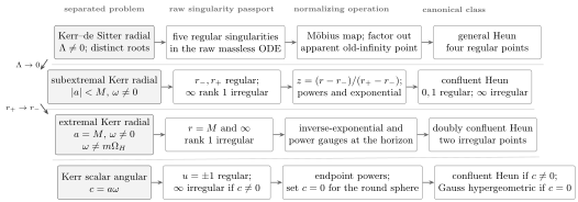
The class changes only after a declared limit and a new singularity audit. The Kerr–de Sitter gauge factors out the apparent regular point inherited from old infinity; $\Lambda\to0$ produces confluent Heun, and the generic horizon collision $r_+\to r_-$ produces a radial doubly confluent equation. The static or synchronous strata are separate degenerations.

A reproducible reduction passport

For any new black-hole wave equation, use this order:

1. State the covariant field equation and the exact perturbation variable.
2. Freeze the metric, coordinate patch, signature, and parameter range.
3. Fix $\ee^{-\ii\omega t+\ii m\phi}$ or its alternative explicitly.
4. Prove, cite, or test separability; do not infer it from stationarity.
5. Print both separated ODEs and one definition of the shared accessory.
6. Record the physical intervals, but factor the leading coefficients over the complex plane.
7. Test every finite point and infinity before naming an ODE class.
8. Give the independent-variable map, scalar gauge, inverse map, and any operator multiplier.
9. Substitute the map into the operator and print the canonical convention.
10. Redo the audit on static, extremal, massless, or near-horizon strata.
11. Only afterward construct the physical local bases and their connection coefficient.

The output of this page ends at step 10. The next two pages add canonical horizon, boundary, angular, and radiation bases and then assemble their Wronskian or recurrence conditions.

What separation has not yet proved

Separation and classification provide	They do not yet provide
Scalar ODEs and an accessory relation	Axis, horizon, infinity, or AdS-boundary normalized bases
Singularities, exponents, and formal ranks	A logarithm branch, frequency sheet, or Stokes sector
A canonical Heun operator tuple	A globally continued Heun solution in a physical normalization
Candidate connection data	A QNM Wronskian or recurrence minimality condition
A master curvature scalar	Metric reconstruction, gauge completion, or a chosen observable
A radial source/response pair	Holographic counterterms and a normalized retarded correlator

For Kerr, the later boundary-function construction has the schematic form

$$E_{\mathrm{ang}}(\omega,A)=0, \qquad E_{\mathrm{rad}}(\omega,A)=0.$$

The first equation selects a smooth angular eigenline and an analytic branch of $A(\omega)$; the second aligns two radial boundary lines. Neither equation is contained in the phrase “confluent Heun.”

Common pitfalls

Inferring separability from symmetry. Stationarity and axisymmetry allow a Fourier decomposition, but they do not remove all $r$–$\theta$ coupling. A hidden-symmetry theorem, direct substitution, or an established separated master equation is still required.

Calling a software function a crosswalk. HeunC argument orders and accessory shifts differ across sources and computer systems. Verify the transformed differential operator term by term.

Taking a singular parameter limit inside a generic tuple. The maps used for $\Lambda\ne0$ or $r_+\ne r_-$ can diverge in the limit. Return to the original equation, scale the coordinate and parameters, and classify again.

Treating the Heun class as a QNM condition. A local special-function representation supplies neither the physical endpoint lines nor their global alignment. Quasinormal frequencies arise only after those choices produce a vanishing connection coefficient.

Exercises

1. Separate the Schwarzschild scalar

Starting from $\Box_g\Phi=0$, compute $\sqrt{-g}$ and derive the angular and radial equations on this page.

Solution

The metric determinant is $g=-r^4\sin^2\theta$, so

$$\Box_g = \frac1{\sqrt{-g}} \partial_\mu \left( \sqrt{-g}\,g^{\mu\nu}\partial_\nu \right)$$

gives the displayed decomposition into time, radial, and spherical parts. After inserting $\Phi=\ee^{-\ii\omega t}\mathcal R(r)Y(\theta,\phi)$ and multiplying by $r^2/(\mathcal RY)$, the $r$-dependent and angular terms must equal a constant. Calling it $L$ yields $-\Delta_{S^2}Y=LY$ and the displayed radial equation. Smoothness on $S^2$ fixes $L=\ell(\ell+1)$.

2. Recover the Regge–Wheeler form

Set $\mathcal R=u/r$ and $\dd r_*/\dd r=f^{-1}$. Show that the first radial derivative disappears and recover $V_\ell$.

Solution

Because $\partial_{r_*}=f\partial_r$,

$$\partial_{r_*}^2u = f^2u''+ff'u'.$$

Substituting $\mathcal R=u/r$ into the rational radial equation cancels the remaining $u'$ term. Since $f'=2M/r^2$, the coefficient of $u$ is

$$V_\ell = f \left[ \frac{\ell(\ell+1)}{r^2} +\frac{f'}r \right] = f \left[ \frac{\ell(\ell+1)}{r^2} +\frac{2M}{r^3} \right].$$

3. Audit all three Schwarzschild singular points

Apply the finite Fuchs tests at $z=0,1$ and use $t=1/z$ at infinity.

Solution

At $z=0$, $zP\to1$ and $z^2Q\to0$. At $z=1$, $(z-1)P\to1$ and $(z-1)^2Q\to\Omega^2$. Both points are regular singular. Under $t=1/z$, the nonzero limit $Q\to\Omega^2$ produces a fourth-order pole in the transformed normal-form coefficient. Thus infinity is rank-one irregular when $\Omega\ne0$.

4. Certify the confluent-Heun tuple

Substitute $\mathcal R=\ee^{\ii\Omega z}(z-1)^{-\ii\Omega}y$ and recover $(q,\alpha,\gamma,\delta,\epsilon)$.

Solution

For $\mathcal R=\ee^h y$ with $h=\ii\Omega z-\ii\Omega\log(z-1)$, the new coefficients are

$$\widetilde P=P+2h', \qquad \widetilde Q=Q+Ph'+h''+(h')^2.$$

Simplification gives

$$\widetilde P = \frac1z +\frac{1-2\ii\Omega}{z-1} +2\ii\Omega,$$

and

$$\widetilde Q = \frac{ (4\Omega^2+2\ii\Omega)z -(L+2\ii\Omega) }{ z(z-1) }.$$

Reading against the declared convention gives the tuple printed in the main text.

5. Expose the static hypergeometric degeneration

Set $\Omega=0$ and verify the parameters $a=-\ell$, $b=\ell+1$, $c=1$.

Solution

The radial equation becomes

$$z(1-z)\mathcal R'' + (1-2z)\mathcal R' + L\mathcal R =0.$$

The Gauss equation has coefficients $c=1$, $a+b+1=2$, and $-ab=L$. Hence $a=-\ell$, $b=\ell+1$. The missing exponential at infinity is precisely the demotion from confluent Heun to hypergeometric.

6. Derive the Kerr horizon exponents

Let $r_h$ be a simple zero of $\Delta$. Derive the indicial equation and rewrite its roots using $\Omega_h$ and $\kappa_h$.

Solution

With $x=r-r_h$,

$$\Delta=\Delta'(r_h)x+O(x^2).$$

The leading standard-form equation is

$$R''+\frac1xR' + \frac{K(r_h)^2}{\Delta'(r_h)^2x^2}R =0.$$

Thus $\rho_h^2+K(r_h)^2/\Delta'(r_h)^2=0$. Since

$$K(r_h) = (r_h^2+a^2) (\omega-m\Omega_h),$$

and $\Delta'(r_h)=2\kappa_h(r_h^2+a^2)$, the roots are the ones printed in the main text. Their labels as ingoing or outgoing still depend on the time and logarithm conventions.

7. Audit the extremal collision and its exception

At $a=M$, show why the radial horizon is irregular for $\omega\ne m\Omega_H$ and why the synchronous locus must be treated separately.

Solution

With $x=r-M$,

$$K(x) = 2M^2(\omega-m\Omega_H) +2M\omega x+\omega x^2.$$

If the constant term is nonzero, $K^2/x^4$ has a fourth-order pole, which is rank one. At $\omega=m\Omega_H$, both that leading term and the inverse-exponential gauge parameter $\beta_K$ vanish. The horizon singularity then has a lower rank and must be reclassified from the specialized equation.

8. Audit the Kerr–de Sitter root map

Verify the images of $r_-$, $r_+$, $r'_-$, and $r=\infty$ under the displayed Möbius map. Why must the $\Lambda\to0$ limit be taken in the full operator?

Solution

Direct substitution gives

$$z(r_-)=0, \qquad z(r_+)=1, \qquad z(r'_-)=\infty.$$

Taking $r\to\infty$ gives the finite value

$$z_\infty = \frac{r_+-r'_-}{r_+-r_-}.$$

As $\Lambda\to0$, the cosmological roots and therefore $z_r$, $z_\infty$, and several Heun parameters diverge. Their divergent pieces combine with the coordinate and scalar gauge to leave finite confluent coefficients. Setting $\Lambda=0$ term by term in the already transformed tuple can erase those combinations, so one must scale the complete differential operator and then reclassify its limit.

9. Separate equation class from Kerr spectrum

Why does a radial confluent-Heun solution at a chosen $(\omega,A)$ not define a Kerr QNM?

Solution

First, smoothness at both angular poles selects an allowed branch of $A(\omega)$. Second, physical radial data select one horizon line and one outer line. A QNM is a common zero of the angular boundary function and the radial connection function. The Heun class identifies neither line and does not discretize $\omega$ by itself.

References

• B. Carter, “Hamilton–Jacobi and Schrödinger Separable Solutions of Einstein’s Equations”, Communications in Mathematical Physics 10 (1968), 280–310. Establishes the separability structure behind the scalar calibration.
• S. A. Teukolsky, “Perturbations of a Rotating Black Hole. I. Fundamental Equations for Gravitational, Electromagnetic, and Neutrino-Field Perturbations”, The Astrophysical Journal 185 (1973), 635–647. Derives the separated master equations for Kerr perturbations.
• E. W. Leaver, “Solutions to a Generalized Spheroidal Wave Equation”, Journal of Mathematical Physics 27 (1986), 1238–1265. Develops convergent solution representations for the confluent-Heun/generalized spheroidal class containing Teukolsky equations.
• H. Suzuki, E. Takasugi, and H. Umetsu, “Perturbations of Kerr–de Sitter Black Holes and Heun’s Equations”, Progress of Theoretical Physics 100 (1998), 491–505. Gives the explicit five-to-four-singularity transformations and the $\Lambda\to0$ confluent limits used above.
• D. Philipp and V. Perlick, “On Analytic Solutions of Wave Equations in Regular Coordinate Systems on Schwarzschild Background”. Audits Schwarzschild radial equations in several coordinate systems and identifies their confluent-Heun singularity structure.
• R. Teixeira da Costa, “Mode Stability for the Teukolsky Equation on Extremal and Subextremal Kerr Spacetimes”, Communications in Mathematical Physics 378 (2020), 705–781. Supplies precise confluent- and doubly-confluent radial operators and their genericity conditions.
• M. Casals and P. Zimmerman, “Perturbations of Extremal Kerr Spacetime: Analytic Framework and Late-Time Tails”, Physical Review D 100 (2019), 124027. Treats the global extremal radial equation, its two rank-one irregular points, and its exceptional frequency structure.
• G. Bonelli, C. Iossa, D. Panea Lichtig, and A. Tanzini, “Irregular Liouville Correlators and Connection Formulae for Heun Functions”, Communications in Mathematical Physics 397 (2023), 635–727. Fixes the residue conventions for the general, confluent, and doubly confluent Heun equations used in the book.