Polynomial Truncation, Hill Determinants, and Quasi-Exact Solvability

A finite tridiagonal determinant can describe three very different objects. It may be the exact characteristic polynomial of an invariant space, an artificial boundary condition imposed at a cutoff, or one member of a normalized sequence converging to an infinite determinant. The same symbol $\det T_N(\lambda)$ does not make these interpretations interchangeable.

This page develops a recurrence-side test that keeps them apart. The central distinction is elementary but decisive:

$$\begin{gathered} \text{finite compatibility} \quad \quad \text{structural closure} \\ \det T_N(\lambda)=0 \quad \quad \gamma_{N+1}(\lambda)=0. \end{gathered}$$

The first condition makes a finite block singular. The second makes the coefficient immediately beyond that block vanish without being set to zero by hand. Only their combination can produce exact termination in the recurrence convention used here.

A status firewall for determinant claims

Before computing, decide which statement is actually being tested.

Reported statement	Evidence required
$T_N(\lambda)$ has a finite-section root	$\det T_N(\lambda)=0$
The recurrence terminates at exact degree $N$	Closure across row $N+1$, finite compatibility, and a nonzero top coefficient
A quasi-exact sector exists	An invariant finite-dimensional function space, not merely one guessed solution
A Hill determinant vanishes	A declared normalization and a convergence theorem for the determinant sequence
An infinite boundary condition is satisfied	The correct minimal, recessive, outgoing, or square-summable sequence line
A physical state exists	The restored gauge plus domain, endpoint, branch, reality, and integrability checks

These implications generally do not reverse. In particular, a stable sequence of finite-section roots is numerical evidence, not a definition of an infinite Hill determinant.

Continuants encode the left boundary exactly

Use the house recurrence

$$\alpha_nu_{n+1} +\beta_nu_n +\gamma_nu_{n-1} =0, \qquad n\geq 0,$$

with

$$u_{-1}=0, \qquad \alpha_0u_1+\beta_0u_0=0.$$

Its principal block on the indices $0,\ldots,N$ is

$$T_N = \begin{pmatrix} \beta_0 & \alpha_0 \\ \gamma_1 & \beta_1 & \alpha_1 \\ & \ddots & \ddots & \ddots \\ && \gamma_{N-1} & \beta_{N-1} & \alpha_{N-1}\\ &&& \gamma_N & \beta_N \end{pmatrix}, \qquad D_N=\det T_N.$$

Set $D_{-1}=1$. Expansion along the last row gives the continuant recurrence

$$\begin{aligned} D_0&=\beta_0,\\ D_n &= \beta_nD_{n-1} -\alpha_{n-1}\gamma_nD_{n-2}, \qquad n\geq1. \end{aligned}$$

The first nontrivial sign audit is

$$\begin{aligned} D_2 ={}& \beta_0\beta_1\beta_2 -\beta_0\alpha_1\gamma_2\\ &-\alpha_0\gamma_1\beta_2. \end{aligned}$$

It is often safer to generate $D_n$ from the two-term continuant update than to ask a general-purpose determinant routine to expand a large symbolic matrix.

The coefficient formula

Fix $u_0\neq0$, normally $u_0=1$, and assume $\alpha_0\alpha_1\cdots\alpha_n\neq0$. The left-normalized solution satisfies

$$u_{n+1} = (-1)^{n+1} \frac{D_n}{ \alpha_0\alpha_1\cdots\alpha_n } u_0.$$

The proof is an induction. The formula for $u_1$ is the row-$0$ condition. Substituting the two preceding formulas into row $n$ produces the continuant recurrence for $D_n$.

Consequently,

$$D_N=0 \quad\Longleftrightarrow\quad u_{N+1}=0$$

on this forward-regular patch. The right-hand statement means only that the solution satisfying the left boundary also satisfies a Dirichlet-type coefficient cutoff at $N+1$. It says nothing yet about row $N+1$ or about infinity.

Exact support is a two-condition theorem

Let $\mathcal E_N$ denote the space of sequences supported on $0,\ldots,N$. The following test also covers exceptional rows where division by an $\alpha_n$ is illegal.

Exact termination theorem

There is a nonzero recurrence solution supported exactly through $N$ if and only if

$$\gamma_{N+1}=0$$

and $\ker T_N$ contains a vector

$$(u_0,\ldots,u_N)^{\mathsf T}$$

with $u_N\neq0$. If the chosen local branch additionally requires $u_0\neq0$, that endpoint condition must be checked as well.

To prove the statement, extend the finite nullvector by zeros. The full recurrence residual is

$$(Tu)_n = \begin{cases} 0, &0\leq n\leq N,\\ \gamma_{N+1}u_N, &n=N+1,\\ 0, &n\geq N+2. \end{cases}$$

Thus the first omitted row contains the entire difference between an exact termination and a cutoff.

If

$$\alpha_0\cdots\alpha_{N-1} \gamma_1\cdots\gamma_N \neq0,$$

then $T_N$ is irreducible tridiagonal. A nonzero nullvector cannot have either endpoint component zero: the first or last row would propagate that zero through the entire vector. On this generic locus the theorem reduces to

$$\gamma_{N+1}=0, \qquad D_N=0.$$

Under the forward assumptions of the coefficient formula, exact degree also requires

$$D_{N-1}\neq0.$$

Irreducibility makes this inequality automatic, but reducible or resonant recurrences require an explicit nullspace calculation.

The invariant wall

In the declared ordered coefficient basis, the closure condition has a direct invariant-subspace meaning:

$$T\mathcal E_N\subseteq\mathcal E_N \quad\Longleftrightarrow\quad \gamma_{N+1}=0.$$

At closure the infinite coefficient operator has block form

$$T = \begin{pmatrix} T_N & *\\ 0 & T_{\mathrm{tail}} \end{pmatrix}.$$

At a parameter value on the closure locus, every larger finite determinant therefore factors pointwise:

$$\det T_M(\lambda_*) = \det T_N(\lambda_*)\, \det T_{N+1:M}(\lambda_*), \qquad M>N.$$

If the wall holds identically in the remaining spectral variable—as it does after a QES degree condition fixes a separate structural parameter—then $\det T_N(\lambda)$ is an analytic factor at every greater depth. If closure occurs only at an isolated $\lambda_*$, the displayed equality is merely pointwise and does not imply polynomial divisibility. An ordinary finite-section root has neither kind of algebraic protection.

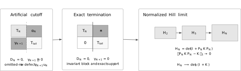
Three operations that must not be conflated. A cutoff deletes a live coupling; exact closure makes the coupling $\gamma_{N+1}$ vanish in the original recurrence; a Hill determinant requires a normalized sequence $H_N$ with a proved limit.

Index conventions

Some references call the terminating coefficient $\alpha_N$ rather than $\gamma_{N+1}$. Their matrix may be transposed, their recurrence may be solved in the opposite direction, or their index may be shifted. Do not memorize the letter. Extend the proposed finite vector by zeros and inspect the first omitted row.

A degree-two biconfluent-Heun checksum

The Heun QES page derives the finite-dimensional sectors of all five DLMF Heun equations. Here one biconfluent example serves a different purpose: it tests the recurrence wall, determinant signs, and polynomial reconstruction at once.

In the DLMF convention,

$$y'' - \left( \frac{\gamma}{z}+\delta+z \right)y' + \frac{\alpha z-q}{z}y =0.$$

After multiplication by $z$, write

$$\mathcal L_0 = zD^2 -(\gamma+\delta z+z^2)D +\alpha z, \qquad \mathcal L_0P=qP.$$

For

$$P(z)=\sum_{n\geq0}c_nz^n,$$

coefficient comparison gives

$$\begin{aligned} &(n+1)(n-\gamma)c_{n+1} -(q+\delta n)c_n\\ &\qquad +(\alpha-n+1)c_{n-1} =0. \end{aligned}$$

Thus

$$\begin{aligned} \alpha_n^{\mathrm{rec}} &=(n+1)(n-\gamma),\\ \beta_n^{\mathrm{rec}} &=-(q+\delta n),\\ \gamma_n^{\mathrm{rec}} &=\alpha-n+1. \end{aligned}$$

The recurrence wall at degree $N$ is

$$\gamma_{N+1}^{\mathrm{rec}} =\alpha-N =0.$$

Choose

$$N=2, \qquad \alpha=2, \qquad \gamma=-\frac12, \qquad \delta=0.$$

Then

$$\mathcal L_0 = zD^2 + \left( \frac12-z^2 \right)D +2z$$

preserves $\mathcal P_2=\operatorname{span}\{1,z,z^2\}$. In that ordered basis its restriction is

$$M_2 = \begin{pmatrix} 0&\frac12&0\\ 2&0&3\\ 0&1&0 \end{pmatrix},$$

and

$$\det(qI-M_2) = q(q^2-4).$$

The three exact eigenpolynomials, normalized by $P(0)=1$, are

$$\begin{array}{c|c} q & P(z)\\ \hline 0 & 1-\dfrac23z^2 \\ 2 & 1+4z+2z^2 \\ -2 & 1-4z+2z^2 \end{array}$$

Direct substitution verifies

$$\mathcal L_0P=qP$$

for all three rows. Because $\gamma_3^{\mathrm{rec}}=0$, the verification continues through the first omitted recurrence row rather than stopping at the $3\times3$ matrix.

This is genuinely quasi-exact: at these fixed parameters $\mathcal P_2$ is invariant, but the operator does not preserve the full flag $\mathcal P_0\subset\mathcal P_1\subset\cdots$. The finite algebraic eigenpairs still need whatever gauge, domain, and endpoint tests belong to the original physical problem.

Continuants are the homogeneous form behind finite fractions

The continued fraction on the previous page and the finite determinant above are not independent algorithms. At fixed depth they are two charts on the same continuant identity.

Allow a general terminal line

$$u_{N+1}=\tau_Nu_N.$$

Substitution into row $N$ replaces only the last diagonal entry:

$$\widehat\beta_N = \beta_N+\alpha_N\tau_N.$$

The choice $\tau_N=0$ is the usual Dirichlet-type coefficient cutoff. An asymptotic tail seed gives a different finite boundary problem and must be named as such.

Define the trailing continuants

$$\begin{aligned} E_{N+1}^{[N]}&=1,\\ E_N^{[N]}&=\widehat\beta_N,\\ E_k^{[N]} &= \beta_kE_{k+1}^{[N]} -\alpha_k\gamma_{k+1}E_{k+2}^{[N]}, \\ &\hspace{34mm}0\leq k<N. \end{aligned}$$

Where the denominator is nonzero, the backward ratio sweep is

$$R_k^{[N]} = \frac{u_k}{u_{k-1}} = -\gamma_k \frac{E_{k+1}^{[N]}}{E_k^{[N]}}.$$

For a zero tail, the finite residual at the left boundary is

$$\begin{aligned} F_0^{[N]} &= \beta_0+\alpha_0R_1^{[N]}\\ &= \beta_0 -\cfrac{\alpha_0\gamma_1}{ \beta_1 -\cfrac{\alpha_1\gamma_2}{ \ddots -\cfrac{\alpha_{N-1}\gamma_N}{\beta_N} } } . \end{aligned}$$

The determinant–fraction identity is

$$F_0^{[N]} = \frac{D_N}{E_1^{[N]}}.$$

Hence $F_0^{[N]}=0$ and $D_N=0$ describe the same finite boundary problem wherever the affine ratio is defined. At a pivot zero retain the division-free equation

$$D_N = \beta_0E_1^{[N]} -\alpha_0\gamma_1E_2^{[N]}.$$

The determinant does not acquire a singularity when one particular continued-fraction chart does.

Two computations, one piece of evidence

A zero-tail continued fraction and the determinant of the corresponding principal block are algebraically identical. Agreement between them checks implementation and chart handling, but it is not an independent validation of the cutoff or of the boundary condition at infinity.

Finite characteristic polynomial or finite section?

The notation $D_N$ hides a structural fork.

Exact finite block

If $\gamma_{N+1}=0$, the underlying operator preserves $\mathcal E_N$. When $\beta_n=b_n-\lambda$ and the remaining entries are independent of $\lambda$,

$$D_N(\lambda) = \det(A_N-\lambda I)$$

is an ordinary degree-$N+1$ characteristic polynomial. Its roots count with algebraic multiplicity. A repeated root may be defective, so the geometric multiplicity and the top coefficient of every eigenvector still need inspection.

In a polynomial basis, this finite block is the algebraic core of a quasi-exactly solvable sector. In a Jaffé, Coulomb-wave, or other nonpolynomial basis, exact support gives a finite basis expansion; it does not automatically give a polynomial in the original coordinate.

Artificial finite section

If $\gamma_{N+1}\neq0$, the equation

$$D_N(\lambda)=0$$

imposes $u_{N+1}=0$ by deleting a live coupling. Extending the nullvector by zeros leaves the explicit defect

$$r_{N+1} = \gamma_{N+1}u_N.$$

This is a legitimate approximation when backed by a finite-section, minimal-tail, or operator-convergence theorem. It is not exact termination.

A determinant sequence

Letting $N$ grow creates a sequence of finite analytic functions. It does not create an infinite determinant by notation:

$$\det T_\infty \neq \text{an automatically defined object}.$$

The index set, reference operator, normalization, parameter domain, and mode of convergence are part of the definition.

What deserves the name Hill determinant?

Classically, a matrix $A=(a_{jk})$ of Hill type is normalized near the identity. A strong sufficient condition is

$$\sum_{j,k} \left| a_{jk}-\delta_{jk} \right| <\infty.$$

Under this hypothesis the corresponding principal determinants converge. The DLMF discussion of infinite determinants uses this condition for Hill-type determinants.

A compact operator $K$ is trace class when its singular values $s_j(K)$ are summable. Their sum is the trace norm,

$$\lVert K\rVert_1 = \sum_j s_j(K).$$

The projection $P_N$ below keeps the first $N+1$ basis vectors. Saying that $K(\lambda)$ is holomorphic means holomorphic as a trace-class-valued function in this norm, not merely entry-by-entry.

For an operator formulation, suppose a declared reference converts the coefficient operator to

$$A(\lambda) = I+K(\lambda),$$

where $K(\lambda)$ is trace class and depends holomorphically on $\lambda$. Then the Fredholm determinant

$$H(\lambda) = \det_{\mathrm F}\!\left(I+K(\lambda)\right)$$

is analytic. If finite projections $P_N$ satisfy

$$\left\| P_NK(\lambda)P_N-K(\lambda) \right\|_1 \longrightarrow0$$

locally uniformly in $\lambda$, then

$$H_N(\lambda) = \det\!\left( I+P_NK(\lambda)P_N \right) \longrightarrow H(\lambda)$$

locally uniformly as well.

This is a clean sufficient framework, not a claim that every recurrence matrix is trace class after naive row division. If only Hilbert–Schmidt control is available, an explicitly declared regularized determinant such as $\det_2$ may be appropriate. Its normalization is different and must not be introduced silently.

Why normalization is mathematical data

Multiplying the $n$th finite row by a nonzero factor $s_n(\lambda)$ changes the determinant by

$$\prod_{n=0}^{N}s_n(\lambda).$$

At fixed $N$, a factor analytic and nonvanishing on the domain leaves the zero set unchanged. As $N\to\infty$, the product may tend to zero, diverge, oscillate, or introduce parameter singularities. Thus two sequences with the same finite zeros can have completely different limits.

Diagonal similarity is safer:

$$\det(S_N^{-1}T_NS_N) = \det T_N.$$

Row scaling is not similarity, and its infinite product must be controlled.

A recurrence-specific convergence theorem

There is a useful elementary criterion that can be checked without invoking the full trace-ideal machinery. Work on a parameter domain $\Omega$ where every $\beta_n(\lambda)$ is nonzero, and normalize the leading continuants by

$$h_n(\lambda) = \frac{D_n(\lambda)}{ \displaystyle\prod_{j=0}^{n}\beta_j(\lambda) }.$$

Set

$$q_n(\lambda) = \frac{ \alpha_{n-1}(\lambda)\gamma_n(\lambda) }{ \beta_{n-1}(\lambda)\beta_n(\lambda) }.$$

Then

$$\begin{aligned} h_{-1}&=1,\\ h_0&=1,\\ h_n&=h_{n-1}-q_nh_{n-2}. \end{aligned}$$

Locally uniform normalized-continuant limit

Assume that the recurrence coefficients are holomorphic on $\Omega$ and that, for every compact set $K\Subset\Omega$,

$$\sum_{n=1}^{\infty} \sup_{\lambda\in K} \left|q_n(\lambda)\right| <\infty.$$

Then $h_n$ converges locally uniformly on $\Omega$ to a holomorphic function $h$.

Here is a short proof. On a fixed compact $K$, let

$$M_n = \max\left( \lVert h_n\rVert_K, \lVert h_{n-1}\rVert_K \right).$$

The recurrence gives

$$M_n \leq \left( 1+\lVert q_n\rVert_K \right)M_{n-1}.$$

The infinite product of the factors on the right is finite, so the sequence $h_n$ is uniformly bounded on $K$. Moreover,

$$\left\| h_n-h_{n-1} \right\|_K \leq \lVert q_n\rVert_K \lVert h_{n-2}\rVert_K.$$

The differences are summable. Hence $h_n$ is uniformly Cauchy on $K$, and Weierstrass’ theorem makes the limit holomorphic.

The criterion is sufficient, not necessary. It is also a chart theorem: zeros of some $\beta_n$ must be covered by another nonvanishing normalization rather than divided through.

What local uniformity buys

Suppose $h\not\equiv0$ and $\Gamma$ is a simple closed contour whose image and interior have compact closure in $\Omega$. If $h$ has no zeros on $\Gamma$, then, for all sufficiently large $N$,

$$\lVert h_N-h\rVert_\Gamma < \min_{\lambda\in\Gamma}|h(\lambda)|.$$

Rouché’s theorem then gives the same number of zeros inside $\Gamma$, counted with multiplicity. In particular:

• an isolated simple zero of $h$ attracts one zero of $h_N$;
• a convergent sequence of zeros of $h_N$ can limit inside $\Omega$ only at a zero of $h$;
• a contour crossing a zero or pole of the chosen normalization must be changed before the theorem applies.

This establishes convergence of determinant zeros. Calling those zeros eigenvalues still requires proof that $h$ represents the intended operator domain or recurrence boundary condition.

A Hill determinant is not the Hill discriminant

The terminology is especially easy to confuse in the Mathieu problem. A Hill determinant is a normalized determinant of a coefficient matrix in a declared Fourier or recurrence sector. The Hill discriminant is

$$\Delta_{\mathrm{Hill}}(a,q) = \operatorname{tr}M_\pi(a,q),$$

the trace of the ODE monodromy over one period. Its Floquet multipliers obey

$$\rho^2 -\Delta_{\mathrm{Hill}}\rho +1 =0.$$

The two objects can encode the same periodic or antiperiodic characteristic values after their sectors and normalizations are fixed, but they are not the same analytic function. The DLMF Floquet discussion defines the discriminant; the later Floquet chapter develops its band interpretation.

Mathieu gives a genuine Hill benchmark

The Mathieu equation

$$y''(x) + \left( a-2q\cos2x \right)y(x) =0$$

provides a transparent infinite example. Work in $L^2([0,\pi],dx)$ on the periodic domain $H^2_{\mathrm{per}}$, restricted to its even subspace. For real $q$, this realization is self-adjoint. An orthonormal basis of the even sector is

$$\begin{aligned} e_0(x)&=\frac1{\sqrt{\pi}},\\ e_n(x)&=\sqrt{\frac2\pi}\cos(2nx), \qquad n\geq1, \end{aligned}$$

In this basis, the operator

$$-\frac{d^2}{dx^2}+2q\cos2x$$

has the Jacobi matrix

$$J_{\mathrm e}(q) = \begin{pmatrix} 0&\sqrt2q\\ \sqrt2q&4&q\\ &q&16&q\\ &&q&36&q\\ &&&\ddots&\ddots \end{pmatrix}.$$

The spectral parameter is $a$:

$$\bigl(J_{\mathrm e}(q)-aI\bigr)c=0.$$

This recurrence does not terminate for $q\neq0$. Its finite matrices are Ritz compressions of a fixed self-adjoint operator when $q$ is real.

A trace-class normalization

Introduce

$$A = \operatorname{diag} \left( 1,5,17,37,\ldots,4n^2+1,\ldots \right)$$

and write

$$\begin{aligned} J_{\mathrm e}(q)-aI &= A^{1/2} \left( I+K_{\mathrm e}(a,q) \right) A^{1/2},\\ K_{\mathrm e}(a,q) &= A^{-1/2} \left[ V(q)-(a+1)I \right] A^{-1/2}, \end{aligned}$$

where $V(q)$ contains the off-diagonal entries of $J_{\mathrm e}(q)$. The diagonal entries of $K_{\mathrm e}$ have absolute size

$$\frac{|a+1|}{4n^2+1},$$

while its off-diagonal entries are, apart from the first $\sqrt2$ factor,

$$\frac{|q|}{ \sqrt{ (4n^2+1) \left(4(n+1)^2+1\right) } }.$$

Both series are summable, locally uniformly in $(a,q)$. Absolute summability of the matrix entries makes $K_{\mathrm e}$ trace class. Therefore

$$H_{\mathrm e}(a,q) = \det_{\mathrm F} \left( I+K_{\mathrm e}(a,q) \right)$$

is a well-defined analytic determinant, and the normalized principal sections are

$$H_{\mathrm e,N}(a,q) = \frac{ \det\left( J_{\mathrm e,N}(q)-aI \right) }{ \displaystyle \prod_{n=0}^{N}(4n^2+1) }.$$

This denominator has no $a$-zeros, so it changes the limit without changing any finite characteristic root.

A high-precision cutoff audit

For $q=1$, the smallest eigenvalue of the section with maximum Fourier index $N$ converges as follows. The values were computed at 80-decimal working precision by diagonalizing the real symmetric sections. Each eigenvector has unit Euclidean norm. The last column reports the magnitude of its final component; for $N\geq1$ it is also the magnitude of the only omitted-row residual because $q=1$.

$N$	Smallest Ritz value $a_0^{[N]}(1)$	Omitted-row residual
$1$	$-0.449489742783178098$	$3.03\times10^{-1}$
$2$	$-0.455129079557300071$	$1.86\times10^{-2}$
$3$	$-0.455138600046465374$	$5.11\times10^{-4}$
$4$	$-0.455138604106786050$	$7.94\times10^{-6}$
$6$	$-0.455138604107413548231109$	$5.47\times10^{-10}$

The comparison reference was generated by solving the Neumann shooting equation below with an 80-decimal Taylor integrator and a secant root solve; it is independent of the finite cosine matrices. At $N=10$, the Ritz value agrees with that reference through 40 decimal places. Rounded to 34 decimal places, the reference is

$$a_0(1) \approx -0.4551386041074135482326331875288859.$$

For real $q$, the Rayleigh–Ritz principle explains why these lowest values decrease toward the true lowest eigenvalue from above. That monotonicity is a self-adjoint variational fact; it does not extend to a complex or nonnormal recurrence.

An independent check integrates the Mathieu equation on $0\leq x\leq\pi/2$ with

$$y(0)=1, \qquad y'(0)=0,$$

and solves

$$y'\!\left(\frac\pi2;a,q\right)=0.$$

The shooting residual tests the differential equation and endpoint condition rather than merely reevaluating the same finite tridiagonal determinant. An independent 80-decimal Taylor-series integration, using degree $80$, a $10^{-65}$ local tolerance, and the unrounded 80-decimal reference value, returned the observed residual

$$\left| y'\!\left(\frac\pi2;a_0(1),1\right) \right| \approx 2.4\times10^{-70}.$$

This is a reproducibility diagnostic, not a rigorous error bound.

What this benchmark proves

The trace-class argument proves convergence of a normalized determinant. The variational argument controls its lowest real root, and shooting checks the ODE interpretation. None of these facts follows from seeing several digits stabilize in the raw determinant.

A self-adjoint cutoff can still be nonterminating

Consider the constant recurrence

$$-u_{n+1} +2xu_n -u_{n-1} =0, \qquad u_{-1}=0, \qquad u_0=1.$$

Its solution is

$$u_n=U_n(x),$$

where $U_n$ is a Chebyshev polynomial of the second kind. The principal determinant is exactly

$$D_N(x) = U_{N+1}(x),$$

with roots

$$x_{k,N} = \cos\left( \frac{k\pi}{N+2} \right), \qquad k=1,\ldots,N+1.$$

Every finite matrix is real symmetric, every root is real and simple, and the roots interlace. Yet

$$\gamma_{N+1}=-1,$$

so none of them is a termination point. At a root,

$$u_{N+1}=0, \qquad u_{N+2}=-u_N\neq0.$$

As $N$ grows, the roots fill $[-1,1]$. To see their infinite-space meaning, let $J$ be the half-line Jacobi operator with unit off-diagonal entries. The sine transform

$$(\mathcal Su)(\theta) = \sqrt{\frac2\pi} \sum_{n=0}^{\infty} u_n\sin\bigl((n+1)\theta\bigr)$$

turns $J$ into multiplication by $2\cos\theta$. Hence its spectrum is the continuous interval $[-2,2]$. The finite roots sample that interval after the scaling $\lambda=2x$; they are not isolated zeros of a raw limiting determinant. Indeed, at $x=0$ the raw sequence $D_N(0)$ cycles through

$$0,-1,0,1,\ldots$$

and has no limit.

This example is an important warning: reality, simplicity, interlacing, and self-adjointness do not convert a finite coefficient-section eigenvalue into polynomial termination or an isolated infinite-spectrum eigenvalue.

Symmetrization: useful protection with a boundary

For real recurrence data, diagonal similarity can sometimes turn the finite tridiagonal matrix into a symmetric one. Suppose

$$\alpha_n\gamma_{n+1}>0.$$

Choose a real $t_n$ with

$$t_n^2 = \alpha_n\gamma_{n+1},$$

and define nonzero $s_n$ recursively by

$$\frac{s_{n+1}}{s_n} = \frac{t_n}{\alpha_n} = \frac{\gamma_{n+1}}{t_n}.$$

Then, for $S=\operatorname{diag}(s_0,\ldots,s_N)$, both off-diagonal entries of $S^{-1}T_NS$ equal $t_n$. Choosing the positive square root gives the standard Jacobi sign convention; another sign choice gives a diagonally similar symmetric matrix with the same finite spectrum.

When, in addition,

$$T_N(\lambda)=J_N-\lambda I$$

for a real irreducible Jacobi matrix $J_N$, its roots are real and simple, and successive principal spectra interlace. The associated characteristic polynomials satisfy a Favard-type three-term recurrence.

These conclusions require the real Jacobi structure. They are not automatic when the spectral parameter enters the off-diagonal coefficients, $\alpha_n\gamma_{n+1}$ changes sign, or the problem is complex and nonnormal. Even in the Jacobi case, the Chebyshev example shows that one still has to distinguish discrete eigenvalues from finite approximants to continuous spectrum.

Nonnormal roots need left and right vectors

Let a simple finite root satisfy

$$T_N(\lambda_*)v=0, \qquad w^*T_N(\lambda_*)=0.$$

For a small matrix perturbation $\delta T_N$, first-order variation gives

$$\delta\lambda = - \frac{ w^*(\delta T_N)v }{ w^*T_N'(\lambda_*)v }.$$

$w$ and $v$ may be rescaled freely, so the invariant denominator diagnostic is

$$\eta_* = \frac{ \left| w^*T_N'(\lambda_*)v \right| }{ \lVert w\rVert_2\lVert v\rVert_2 }.$$

A small $\eta_*$ signals a sensitive root. At a computed approximation $\widehat\lambda$, a tiny value of $|\det T_N(\widehat\lambda)|$ does not rule out this sensitivity. In the special pencil $T_N=A_N-\lambda I$, the condition contains the familiar factor

$$\frac{\lVert w\rVert_2\lVert v\rVert_2}{ |w^*v| }.$$

For a normalized Hermitian eigenpair one may take $w=v$, and this factor is one. For a highly nonnormal section it can be enormous. Depth stability must therefore be paired with precision tests, left–right conditioning, and an independent formulation.

A decision workflow for recurrence determinants

1. Declare the recurrence and basis. Record the sign convention, starting row, gauge, coordinate, and the analytic meaning of finite support.
2. Inspect the first omitted row. Determine whether the original coefficients give $\gamma_{N+1}=0$. Do not infer closure from a truncated matrix.
3. Build the finite block without unsafe division. Use continuants or a rank-revealing factorization, and inspect every nullvector when an interior coefficient vanishes.
4. Name the finite boundary. A zero tail, asymptotic seed, and matching condition define different finite approximants.
5. Choose the correct interpretation. With a wall, compute an exact invariant block. Without one, state a normalization and the theorem connecting finite sections to the intended infinite object.
6. Track zeros and poles together. Use homogeneous continued-fraction pairs or determinant identities at affine chart poles.
7. Count roots on contours. Local uniform convergence plus Rouché’s theorem is stronger than matching a few decimals along one root branch.
8. Test the full problem. Check the first omitted row, the recurrence or ODE residual, the infinite boundary line, and the restored physical domain independently.

For a quasi-exact claim, also verify that the finite space is preserved before selecting an eigenvector. For a Hill claim, report the normalized function, not just a list of roots.

Common pitfalls

Calling one vanished coefficient termination. The condition $D_N=0$ enforces a finite right boundary, whereas $\gamma_{N+1}=0$ closes the coefficient space. Exact termination needs both, plus a nonzero degree-$N$ component.

Stopping after closure. A vanishing omitted-row coupling makes $\mathcal E_N$ invariant but does not make the restricted operator singular at the chosen parameter. The finite characteristic equation still has to be solved.

Dividing through an exceptional row. If an $\alpha_n$, $\beta_n$, or $\gamma_n$ vanishes, ratio propagation can lose a valid solution or invent a pole. Return to the finite nullspace or to homogeneous projective pairs.

Calling a raw limit a Hill determinant. Finite determinants can grow, decay, or oscillate solely because of row normalization. State the reference operator and prove convergence before writing an infinite determinant.

Double-counting equivalent checks. A zero-tail fraction and its continuant determinant encode the same finite boundary. Use a different basis, ODE shooting, a Wronskian, or a certified contour count for an independent check.

Equating QES with physical solvability. A finite invariant space gives exact algebraic candidates. It does not decide square integrability, single-valuedness, endpoint regularity, a Stokes sector, or whether the physical energy coincides with the accessory parameter.

Exercises

1. Derive the coefficient–continuant identity

Starting from $u_{-1}=0$, prove

$$u_{n+1} = (-1)^{n+1} \frac{D_n}{ \alpha_0\cdots\alpha_n }u_0$$

whenever the denominator is nonzero.

Solution

For $n=0$, row $0$ gives

$$u_1 = -\frac{\beta_0}{\alpha_0}u_0 = -\frac{D_0}{\alpha_0}u_0.$$

Assume the formula at the two preceding indices. Row $n$ gives

$$u_{n+1} = -\frac{ \beta_nu_n+\gamma_nu_{n-1} }{\alpha_n}.$$

After substitution and a common denominator, the numerator becomes

$$\beta_nD_{n-1} -\alpha_{n-1}\gamma_nD_{n-2} = D_n.$$

The alternating sign advances by one, completing the induction.

2. Expose a fake termination

Take

$$u_{n+1}-qu_n+u_{n-1}=0, \qquad u_{-1}=0, \qquad u_0=1.$$

Truncate at $N=1$. Find the finite roots and evaluate the first omitted-row residual after extending the finite vector by zeros.

Solution

The finite block and determinant are

$$T_1 = \begin{pmatrix} -q&1\\ 1&-q \end{pmatrix}, \qquad D_1=q^2-1.$$

Thus $q=\pm1$. Row $0$ gives $u_1=q$, and the cutoff has $u_2=0$. The extended vector fails at row $2$ by

$$r_2 = \gamma_2u_1 = q \neq0.$$

The finite roots are genuine Dirichlet-section roots, but $\gamma_2=1$ prevents termination.

3. Audit an exceptional biconfluent row

In the biconfluent recurrence, set

$$N=1, \qquad \alpha=1, \qquad \gamma=0.$$

Show that, for $\delta\neq0$, the invariant block has the two eigenpairs

$$q=0,\quad P=\delta+z, \qquad q=-\delta,\quad P=z.$$

What happens at $\delta=0$?

Solution

In the basis $(1,z)$ the restricted operator is

$$M_1 = \begin{pmatrix} 0&0\\ 1&-\delta \end{pmatrix}.$$

Its characteristic polynomial is $q(q+\delta)$. At $q=0$, a nullvector of $M_1$ is $(\delta,1)^{\mathsf T}$; at $q=-\delta$, an eigenvector is $(0,1)^{\mathsf T}$. The latter branch is invisible to the normalization $c_0=1$.

When $\delta=0$, the matrix is a nonzero nilpotent Jordan block. The characteristic root $q=0$ has algebraic multiplicity two but only one eigenline, spanned by $z$; the constant basis vector is a generalized eigenvector. Determinant multiplicity is not geometric multiplicity.

4. Recover the finite continued fraction

Starting from the trailing continuants $E_k^{[N]}$, prove

$$R_k^{[N]} = -\gamma_k \frac{E_{k+1}^{[N]}}{E_k^{[N]}}$$

and

$$F_0^{[N]} = \frac{D_N}{E_1^{[N]}}$$

for a zero tail. Explain what remains valid when $E_1^{[N]}=0$.

Solution

The terminal ratio is

$$R_N^{[N]} = -\frac{\gamma_N}{\beta_N} = -\gamma_N \frac{E_{N+1}^{[N]}}{E_N^{[N]}}.$$

If the formula holds one step to the right, the Riccati map gives

$$\begin{aligned} R_k^{[N]} &= -\frac{\gamma_k}{ \beta_k+\alpha_kR_{k+1}^{[N]} }\\ &= -\gamma_k \frac{E_{k+1}^{[N]}}{ \beta_kE_{k+1}^{[N]} -\alpha_k\gamma_{k+1}E_{k+2}^{[N]} }, \end{aligned}$$

which is the required formula. At the left boundary,

$$\begin{aligned} F_0^{[N]} &= \beta_0 -\alpha_0\gamma_1 \frac{E_2^{[N]}}{E_1^{[N]}}\\ &= \frac{ \beta_0E_1^{[N]} -\alpha_0\gamma_1E_2^{[N]} }{E_1^{[N]}} = \frac{D_N}{E_1^{[N]}}. \end{aligned}$$

If $E_1^{[N]}=0$, the affine fraction is outside its chart. The cross-multiplied continuant identity for $D_N$ remains valid.

5. Prove the Chebyshev counterexample

Show that the constant tridiagonal determinant satisfies

$$D_N(x)=U_{N+1}(x),$$

derive its roots, and verify that no root gives exact support.

Solution

The continuant starts with

$$D_{-1}=1, \qquad D_0=2x,$$

and obeys

$$D_N=2xD_{N-1}-D_{N-2}.$$

These are precisely the initial values and recurrence of $U_{N+1}(x)$. Since

$$U_m(\cos\theta) = \frac{\sin((m+1)\theta)}{\sin\theta},$$

the roots are

$$x_{k,N} = \cos\left( \frac{k\pi}{N+2} \right).$$

The closure coefficient remains $\gamma_{N+1}=-1$. At a finite root the next full recurrence row gives $u_{N+2}=-u_N\neq0$, so the zero at $u_{N+1}$ does not propagate.

6. Verify the Mathieu normalization

Prove that the displayed $K_{\mathrm e}(a,q)$ has absolutely summable matrix entries on compact parameter sets. Then show that the full residual of a normalized $N$th finite eigenvector has norm $|q c_N|$ for $N\geq1$.

Solution

On a compact set, $|a+1|$ and $|q|$ are bounded. The diagonal series is bounded by a constant times

$$\sum_{n=0}^{\infty}\frac1{4n^2+1},$$

and the two off-diagonal series are bounded by a constant times

$$\sum_{n=1}^{\infty} \frac1{ \sqrt{ (4n^2+1) \left(4(n+1)^2+1\right) } }.$$

Both converge by comparison with $\sum n^{-2}$; the finitely many initial entries do not matter. Hence the matrix entries are absolutely summable, uniformly on compact parameter sets.

Extend a finite eigenvector $(c_0,\ldots,c_N)$ by zeros. All retained rows vanish. The only new nonzero row is $N+1$, where the Jacobi coupling gives

$$r_{N+1}=q c_N.$$

All later rows vanish, so the full $\ell^2$ residual norm is $|q c_N|$.

7. Derive the nonnormal root perturbation

Let $T(\lambda_*)v=0$ and $w^*T(\lambda_*)=0$, with $w^*T'(\lambda_*)v\neq0$. Derive the first-order displacement caused by a small perturbation $\delta T$.

Solution

Linearize the perturbed null-vector equation:

$$\left[ T(\lambda_*) +T'(\lambda_*)\delta\lambda +\delta T \right] (v+\delta v) =0.$$

Discard second-order terms and multiply on the left by $w^*$. The term $w^*T(\lambda_*)\delta v$ vanishes, leaving

$$w^*T'(\lambda_*)v\,\delta\lambda +w^*(\delta T)v =0.$$

Therefore

$$\delta\lambda = - \frac{ w^*(\delta T)v }{ w^*T'(\lambda_*)v }.$$

References

• NIST Digital Library of Mathematical Functions, §1.3(iii), “Infinite Determinants”, for the classical Hill-type convergence condition.
• NIST Digital Library of Mathematical Functions, §3.10, “Continued Fractions”, for convergents, continuants, and stable backward evaluation.
• NIST Digital Library of Mathematical Functions, §28.4, “Fourier Series”, §28.29, “Hill’s Equation”, and §28.34, “Methods of Computation”, for Mathieu recurrences, the Hill discriminant, and characteristic values.
• NIST Digital Library of Mathematical Functions, §31.5, “Heun Polynomials” and §31.12, “Confluent Forms”, for finite Heun matrices and the biconfluent convention.
• W. Gautschi, “Computational Aspects of Three-Term Recurrence Relations”, SIAM Review 9 (1967), 24–82, for minimal solutions, continued fractions, and recurrence stability.
• E. W. Leaver, “An Analytic Representation for the Quasi-Normal Modes of Kerr Black Holes”, Proceedings of the Royal Society A 402 (1985), 285–298, for the recurrence boundary condition at infinity and its continued-fraction implementation.
• A. V. Turbiner, “Quasi-Exactly-Solvable Problems and $\mathfrak{sl}_2$ Algebra”, Communications in Mathematical Physics 118 (1988), 467–474, for finite-dimensional invariant spaces in quasi-exact solvability.
• C. M. Bender and G. V. Dunne, “Quasi-Exactly Solvable Systems and Orthogonal Polynomials”, Journal of Mathematical Physics 37 (1996), 6–11, for critical spectral polynomials and their recurrence structure.
• B. Simon, “Notes on Infinite Determinants of Hilbert Space Operators”, Advances in Mathematics 24 (1977), 244–273, for trace ideals, Fredholm determinants, and regularized determinants.
• F. Bornemann, “On the Numerical Evaluation of Fredholm Determinants”, Mathematics of Computation 79 (2010), 871–915, for projection convergence in trace norm and determinant computation.
• M. A. Johnson and K. Zumbrun, “Convergence of Hill’s Method for Nonselfadjoint Operators”, SIAM Journal on Numerical Analysis 50 (2012), 64–78, for a modified-Fredholm-determinant proof of Hill-method convergence beyond the self-adjoint setting.
• E. B. Davies and M. Plum, “Spectral Pollution”, IMA Journal of Numerical Analysis 24 (2004), 417–438, for false limiting spectra in projection methods.

Next page

The next page fixes the operator and boundary lines, constructs the Green function, and shows when a recurrence characteristic function produces a resolvent pole or a quasinormal-mode condition. The determinant zero then acquires spectral meaning rather than merely algebraic or numerical status.