Polynomial, Algebraic, and Quasi-Exactly Solvable Sectors

Series termination in a Heun equation is not a lucky cancellation at the end of a recurrence. After denominators are cleared, the differential operator preserves a finite-dimensional polynomial space. One parameter closes that space; the accessory parameter is then an eigenvalue of the resulting finite matrix. This viewpoint works without change for the general, confluent, doubly confluent, biconfluent, and triconfluent equations.

It also prevents three common conflations. A polynomial is a kind of function, algebraicity is a finite-branching property, and quasi-exact solvability is a property of an operator and a selected invariant space. They overlap, but none is a synonym for the others.

Five different claims live in the special sector

The following vocabulary will be kept separate throughout the book.

Claim	Certificate	What it does not imply
Polynomial solution	$y=P_N(z)$ with $\deg P_N=N$	A second polynomial solution or finite monodromy
Quasi-polynomial solution	$y=\chi(z)P_N(z)$ for a declared gauge $\chi$	Algebraicity when $\chi$ contains a genuine exponential
Algebraic solution	$F(z,y)=0$ for some nonzero polynomial $F$	That the whole two-dimensional solution space is algebraic
Liouvillian solution	Construction by algebraic extensions, exponentials, and quadratures	A polynomial representation or finite branching
Quasi-exact solvability	After a fixed coordinate and gauge, the spectral operator preserves an explicit space such as $\chi\mathcal P_N$	The complete spectrum or even an admissible physical state

A polynomial is algebraic and Liouvillian. A power-gauged polynomial with rational powers is algebraic on a finite branched cover. An exponential-gauged polynomial is often Liouvillian but is normally not algebraic. The term QES sector refers to the invariant space that produces such functions, not to their analytic type after every gauge is restored. On this page, quasi-polynomial always means a declared elementary gauge times a polynomial; elsewhere the same word can also mean a finite sum of other special functions.

Two conditions, not one

A degree-closing relation such as $\alpha=-N$ is only the first condition. The accessory parameter must also satisfy a finite spectral equation. At exceptional parameters, the resulting eigenvector can have degree below $N$, so its highest coefficient must be checked as well.

Termination is an invariant-subspace theorem

Let

$$\mathcal P_N = \operatorname{span}_{\mathbb C} \{1,z,\ldots,z^N\}, \qquad D=\frac{\dd}{\dd z}.$$

Write a cleared canonical equation as

$$\mathcal L_0 P=qP,$$

where $q$ is the accessory parameter. Suppose that

$$\mathcal L_0z^k = r_kz^{k+1} +\text{terms of degree at most }k.$$

Every monomial below the top already maps into $\mathcal P_N$. Therefore

$$\mathcal L_0\mathcal P_N \subseteq \mathcal P_N \quad\Longleftrightarrow\quad r_N=0.$$

In the ordered monomial basis, let

$$M_N = \left. \mathcal L_0 \right|_{\mathcal P_N}.$$

Then a nonzero polynomial of degree at most $N$ exists precisely when

$$\det(M_N-qI)=0.$$

The coefficient vector of the polynomial is an eigenvector. The characteristic equation has degree $N+1$ counting algebraic multiplicity, but its roots need not be distinct and a repeated root need not have a full set of eigenvectors.

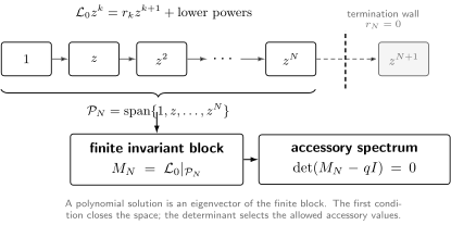
The finite-dimensional mechanism behind Heun termination. The highest raising coefficient $r_N$ closes $\mathcal P_N$; the finite matrix then selects $q$. These are logically separate tests.

Multiplying an ODE by its common denominator does not change its solutions away from the poles. A candidate eigenpolynomial must nevertheless be substituted back into the original meromorphic equation. This final check catches removable-singularity assumptions and degenerate parameter strata.

One calculation closes all five Heun families

Use exactly the DLMF conventions fixed on the confluence page. After clearing denominators, the five operators are as follows.

For the general equation,

$$\begin{aligned} \mathcal L_0^{\mathrm G} ={}& z(z-1)(z-a)D^2\\ &+ \bigl[ \gamma(z-1)(z-a) +\delta z(z-a)\\ &\quad +\epsilon z(z-1) \bigr]D +\alpha\beta z. \end{aligned}$$

For the confluent equation,

$$\begin{aligned} \mathcal L_0^{\mathrm C} ={}& z(z-1)D^2\\ &+ \bigl[ \gamma(z-1)+\delta z \bigr]D \\ &+ \epsilon z(z-1)D +\alpha z. \end{aligned}$$

For the doubly confluent equation,

$$\mathcal L_0^{\mathrm D} = z^2D^2 +(\delta+\gamma z+z^2)D +\alpha z.$$

For the biconfluent and triconfluent equations,

$$\begin{aligned} \mathcal L_0^{\mathrm B} &= zD^2 -(\gamma+\delta z+z^2)D +\alpha z, \\ \mathcal L_0^{\mathrm T} &= D^2 +(\gamma+z)zD +\alpha z. \end{aligned}$$

Only the coefficient of the highest possible power is needed to test invariance:

Class	Raising coefficient in $\mathcal L_0z^k$	Closure of $\mathcal P_N$
GHE	$r_k=(k+\alpha)(k+\beta)$	$\alpha=-N$ or $\beta=-N$
CHE	$r_k=\epsilon k+\alpha$	$\alpha=-N\epsilon$
DCHE	$r_k=k+\alpha$	$\alpha=-N$
BHE	$r_k=\alpha-k$	$\alpha=N$
THE	$r_k=k+\alpha$	$\alpha=-N$

This table is convention-sensitive. For example, the plus sign $\alpha=N$ in the biconfluent row follows from the minus sign in front of the DLMF derivative coefficient. Translating a closure condition to Maple or Wolfram requires the parameter crosswalk, not a function-name substitution.

The constant sector is a useful checksum. At $N=0$, impose $\alpha=0$ in CHE, DCHE, BHE, or THE, or impose $\alpha=0$ or $\beta=0$ in GHE. Then $P_0=1$ and $q=0$.

There are two important exact-degree refinements:

• In GHE, the choice $\alpha=-N$ can contain a smaller invariant space if also $\beta=-m$ for some $0\leq m<N$, and conversely.
• For CHE with $\epsilon\neq0$, and for DCHE, BHE, and THE, a nonzero eigenpolynomial in the $N$ sector must have exact degree $N$. If $\epsilon=0$ and $\alpha=0$, the CHE operator preserves the whole polynomial flag; this is a rank-degenerate exactly solvable limit rather than an isolated QES sector.

The doubly confluent row is especially instructive. Both endpoints are generically irregular, so there is no generic Frobenius-normalized origin function. That fact does not prohibit exceptional polynomial solutions: when $\alpha=-N$ and the finite $q$ equation holds, the meromorphic ODE has a polynomial solution on $\mathbb C^\times$ that extends as an entire function.

General-Heun polynomials from the recurrence

Take the general-Heun branch $\alpha=-N$; the branch $\beta=-N$ is symmetric. Write

$$P(z)=\sum_{n=0}^{N}c_nz^n, \qquad c_{-1}=c_{N+1}=0.$$

The coefficient of $z^n$ in $(\mathcal L_0^{\mathrm G}-q)P$ gives

$$\begin{aligned} &a(n+1)(n+\gamma)c_{n+1} -(q+Q_n)c_n\\ &\qquad+ (n+\alpha-1)(n+\beta-1)c_{n-1} =0,\\ &Q_n = n\left[ (1+a)(n+\gamma-1) +a\delta+\epsilon \right]. \end{aligned}$$

For $n=0,\ldots,N$, these relations form the finite accessory eigenproblem. The coefficient equation at $n=N+1$ reduces to $(N+\alpha)(N+\beta)c_N=0$ and is automatic on the branch $\alpha=-N$; all higher equations vanish. In the generic origin normalization $c_0=1$,

$$c_1=\frac{q}{a\gamma}.$$

When $\gamma\in\{0,-1,-2,\ldots\}$, that normalization may fail even though the finite operator problem remains meaningful. One should solve for a nonzero coefficient vector first and normalize afterward.

For $N=1$, set $\alpha=-1$. The Fuchs relation gives

$$\beta=\gamma+\delta+\epsilon.$$

With

$$K = \gamma(1+a)+a\delta+\epsilon,$$

the degree-one accessory equation and a convenient unnormalized eigenpolynomial are

$$\begin{aligned} q(q+K)+a\gamma\beta&=0,\\ P_1(z)&=a\gamma+qz. \end{aligned}$$

This is the smallest nontrivial Heun polynomial. The first relation $\alpha=-1$ makes $\mathcal P_1$ invariant; the quadratic in $q$ chooses the eigenline inside that two-dimensional space.

On the unobstructed normalized-series locus, the finite eigenpolynomials are the DLMF Heun polynomials

$$\begin{aligned} P_{N,m}(z) &= H\!\ell\!\left( \begin{gathered} a,q_{N,m};-N,\beta,\\ \gamma,\delta;z \end{gathered} \right),\\ m&=0,\ldots,N. \end{aligned}$$

They are analytic at all three finite singularities $0$, $1$, and $a$. Outside that generic normalization locus, “polynomial solution” remains the safe operator-level statement.

In the Heine–Stieltjes sign convention $AP''+BP'-VP=0$, the cubic $A$ and quadratic $B$ are fixed, while $V=q-\alpha\beta z$ is the degree-one Van Vleck polynomial. The classical electrostatic interpretation concerns the roots of $P_N$, with the Van Vleck parameter selecting admissible equilibria, and needs additional real positivity assumptions. The finite-dimensional algebra above is valid over $\mathbb C$ without them.

Zeros obey a finite equilibrium system

Suppose $\alpha=-N$ and a monic eigenpolynomial has distinct roots away from the finite singularities:

$$P_N(z)=\prod_{i=1}^{N}(z-z_i).$$

Evaluating the ODE at each root gives the Bethe–Stieltjes equations

$$2\sum_{\substack{j=1\\j\neq i}}^N \frac1{z_i-z_j} + \frac{\gamma}{z_i} + \frac{\delta}{z_i-1} + \frac{\epsilon}{z_i-a} =0.$$

The accessory parameter is recovered from the sum of roots:

$$\begin{aligned} q ={}& (\beta+N-1) \sum_{i=1}^{N}z_i\\ &- N\left[ (1+a)(N-1+\gamma) +a\delta+\epsilon \right]. \end{aligned}$$

This root description is equivalent to the coefficient eigenproblem only on the stated simple-root locus. Collisions with one another or with a singular point are degenerate cases and should be handled by the finite matrix instead.

A degree-one atlas for the confluent descendants

The same calculation provides a useful sign audit for every confluent form. At generic parameter values the degree-one sectors are:

Class	Closure condition	Accessory equation
CHE	$\alpha=-\epsilon$	$q[q-(\gamma+\delta-\epsilon)]-\epsilon\gamma=0$
DCHE	$\alpha=-1$	$q^2-\gamma q+\delta=0$
BHE	$\alpha=1$	$q(q+\delta)+\gamma=0$
THE	$\alpha=-1$	$q(q-\gamma)=0$

Convenient representatives are

$$\begin{array}{c|c} \text{class}&P_1(z)\\ \hline \mathrm{CHE}&\gamma-qz\\ \mathrm{DCHE}&\delta+qz\\ \mathrm{BHE}&\gamma-qz \end{array}$$

For THE the two generic eigenpairs are

$$\begin{aligned} q=0 &: & P_1(z)&=z+\gamma, \\ q=\gamma &: & P_1(z)&=z. \end{aligned}$$

If $\gamma=0$, the two accessory roots coalesce and the finite matrix has only one eigenline. This elementary example is enough to disprove the frequent assertion that a degree-$N$ termination condition always produces $N+1$ distinct polynomial solutions. A generalized eigenvector satisfies

$$(\mathcal L_0^{\mathrm T}-q)P^{(1)} = P^{(0)},$$

so it solves an inhomogeneous equation and is not a second eigenpolynomial.

These are operator eigenpolynomials. A package’s named origin-normalized triconfluent function need not select either eigenvector without an additional initial-data match.

Index gauges generate quasi-polynomial sectors

Strict polynomials are only one gauge sector. At the three finite singularities of GHE, choose

$$\begin{aligned} s_0&\in\{0,1-\gamma\},\\ s_1&\in\{0,1-\delta\},\\ s_a&\in\{0,1-\epsilon\}, \end{aligned}$$

and set

$$y(z) = z^{s_0}(z-1)^{s_1}(z-a)^{s_a}u(z).$$

After a branch and cuts are fixed, $u$ satisfies another general-Heun equation. If

$$S=s_0+s_1+s_a,$$

its transformed parameters are

$$\begin{aligned} \gamma'&=\gamma+2s_0, \\ \delta'&=\delta+2s_1, \\ \epsilon'&=\epsilon+2s_a, \\ \alpha'&=\alpha+S, \\ \beta'&=\beta+S, \\ q' &= q+(a\delta+\epsilon)s_0 +a\gamma s_1\\ &\quad +\gamma s_a +2as_0s_1+2s_0s_a. \end{aligned}$$

Whenever $\alpha'=-N$ or $\beta'=-N$ and the transformed accessory determinant vanishes, $u=P_N$ and the original solution is

$$y(z) = z^{s_0}(z-1)^{s_1}(z-a)^{s_a}P_N(z).$$

Thus the three binary index choices generate eight finite-singularity gauge sectors before Möbius permutations are considered. The displayed $q'$ is the accessory parameter to use in the transformed finite determinant; it does not stay fixed merely because the exponents have shifted.

The analytic label depends on the gauge:

• if every $s_j$ is a nonnegative integer, $y$ is a polynomial;
• if every $s_j$ is an integer but some are negative, $y$ is rational and becomes polynomial only if zeros of $P_N$ cancel every pole;
• if every $s_j$ is rational and some are noninteger, $y$ is algebraic on a finite branched cover;
• generic irrational powers give infinite branching;
• a genuine exponential gauge in a confluent equation normally gives a nonalgebraic quasi-polynomial.

The transformation page tracks the associated branches, Wronskians, and continuation paths.

Four exponential gauges of DCHE

The doubly confluent equation makes the exponential part of “quasi-polynomial” explicit. Assume $\delta\neq0$, absorb any zero of $P$ at the origin into its power, fix a branch of $z^r$, and set

$$y(z) = \exp\left( sz+\frac tz \right)z^rP(z).$$

Direct conjugation shows that the absence of degree-$N+2$, $z^{-1}$, and $z^{-2}$ obstructions leaves four gauges:

Gauge $\chi(z)$	Closure condition	Accessory value for the finite block
$1$	$\alpha=-N$	$\widehat q=q$
$\ee^{-z}$	$\alpha=N+\gamma$	$\widehat q=q+\delta$
$\ee^{\delta/z}z^{2-\gamma}$	$\alpha=\gamma-N-2$	$\widehat q=q+\gamma+\delta-2$
$\ee^{-z+\delta/z}z^{2-\gamma}$	$\alpha=N+2$	$\widehat q=q+\gamma-2$

In each row, the remaining condition is

$$\widehat q \in \operatorname{Spec} \left( M_N^{(\chi)} \right),$$

where $M_N^{(\chi)}$ is the conjugated operator restricted to $\mathcal P_N$. The four rows pair the two formal exponential choices at zero with the two at infinity. When $\delta=0$, the origin becomes rank-degenerate and this atlas must be reclassified rather than used by continuity.

Algebraicity is a global finite-branching condition

A local solution branch is algebraic over $\mathbb C(z)$ if a nonzero polynomial $F$ satisfies

$$F\bigl(z,y(z)\bigr)=0.$$

Analytic continuation then produces only finitely many branches. A single Heun polynomial supplies one invariant line with trivial continuation, but it says almost nothing about the complementary solution. If $y_1$ is known, reduction of order gives

$$y_2(z) = y_1(z) \int^z \frac{ \exp\left(-\int^s p(t)\,\dd t\right) }{ y_1(s)^2 } \dd s$$

for $y''+p(z)y'+r(z)y=0$. The quadrature may generate logarithms or more general transcendental functions even when $y_1$ is a polynomial.

For a regular-singular equation on the sphere with coefficients in $\mathbb C(z)$, a full basis of algebraic solutions exists if and only if the linear monodromy group is finite. Finite projective monodromy controls the ratio of two solutions; its scalar character, equivalently the Wronskian character, must still be audited before claiming that the individual solutions are algebraic. Klein’s pullback principle relates the finite-projective-monodromy problem, up to a radical gauge and removal of apparent singularities, to a finite-monodromy hypergeometric equation.

A practical construction has the form

$$y(z) = \chi(z)\, {}_2F_1 \left( A,B;C;\phi(z) \right),$$

where $\phi$ is rational and $\chi$ is a radical gauge. Pullback singularities come from inverse images of $0$, $1$, and $\infty$; ramification over an ordinary hypergeometric point can also create an apparent pullback singularity. Some candidate singularities become ordinary or apparent after the gauge. Belyi maps, whose critical values lie in $\{0,1,\infty\}$, organize many classified hypergeometric-to-Heun reductions. If the source hypergeometric solutions are algebraic, the radical pullback remains algebraic.

A particularly clean normalized-germ identity is

$$\begin{aligned} &H\!\ell \left( \frac12,2AB; 2A,2B,C,C; x \right)\\ &\qquad= {}_2F_1 \left( A,B;C;4x(1-x) \right). \end{aligned}$$

For nonexceptional $C$, this is a quadratic hypergeometric-to-Heun identity of normalized germs near $x=0$; exceptional values are handled only after analytic continuation or a parameter limit. For generic $A$, $B$, and $C$, both sides remain transcendental.

Now set $B=C$. The elementary identity ${}_2F_1(A,C;C;u)=(1-u)^{-A}$ gives

$$\begin{aligned} &H\!\ell\!\left( \begin{gathered} \frac12,2AC;\\ 2A,2C,C,C;x \end{gathered} \right)\\ &\qquad= (1-2x)^{-2A}. \end{aligned}$$

For example, $A=1/3$ produces the algebraic, nonpolynomial germ $(1-2x)^{-2/3}$ on the branch equal to $1$ at the origin. This one algebraic solution still says nothing by itself about the complementary solution.

Three tests must not be weakened:

1. Rational local exponent differences are necessary for finite local projective monodromy, but not sufficient for finite global monodromy.
2. An apparent singularity has trivial or scalar local monodromy after the relevant gauge; it does not force the other monodromy generators to be finite.
3. One algebraic solution makes the monodromy reducible on a finite cover; it does not make the full representation finite.

These finite-monodromy statements are Fuchsian. They cannot be transferred unchanged to a genuinely confluent equation, where exponential factors and Stokes matrices are additional global data.

Hidden sl₂ explains the QES language

On $\mathcal P_N$, define

$$\begin{aligned} J^-&=D,\\ J^0&=zD-\frac N2,\\ J^+&=z^2D-Nz. \end{aligned}$$

Their action on a monomial is

$$\begin{aligned} J^-z^k&=kz^{k-1},\\ J^0z^k&=\left(k-\frac N2\right)z^k,\\ J^+z^k&=(k-N)z^{k+1}. \end{aligned}$$

In particular, $J^+z^N=0$. These operators realize $\mathfrak{sl}_2$ and preserve $\mathcal P_N$. Quadratic polynomials in the three generators give the standard one-variable $\mathfrak{sl}_2$-algebraic second-order QES operators.

The cleared Heun operators above enter this class when their closure condition is imposed. The condition depends on the selected $N$, so it usually produces one invariant space, not the entire flag

$$\mathcal P_0 \subset \mathcal P_1 \subset \mathcal P_2 \subset\cdots.$$

Preservation of one member is the quasi-exact statement. Preservation of a full nested flag, with compatible parameters, is the stronger exactly solvable situation.

In a Schrödinger reduction, the physical wavefunction commonly has the form

$$\Psi(x) = \chi\bigl(z(x)\bigr) P_N\bigl(z(x)\bigr).$$

The finite matrix supplies a finite set of candidate spectral values and wavefunctions. It does not decide whether $\Psi$ is single-valued on the physical domain, square-integrable, regular at an endpoint, or recessive in the required Stokes sectors. Those boundary and sector conditions remain part of the spectral problem. The physical energy may also enter several canonical parameters rather than coincide with $q$.

What comes next

This page identifies the exact finite block and its characteristic equation. Stable recurrences, continuants, Hill determinants, root conditioning, and numerical certification belong to the next chapter on Wronskians and direct computation. Here $\det(M_N-qI)$ is an ordinary finite characteristic polynomial because $\mathcal P_N$ closes exactly. A Hill determinant belongs to an infinite recurrence and is defined through a limiting sequence of truncations; it is not another name for this finite determinant.

An audit workflow for a claimed special solution

1. Declare the equation convention. Record the exact ODE and ordered parameter tuple.
2. Choose the coordinate and gauge. Decide whether the finite object is $P_N(z)$ or $\chi(z)P_N(z)$, and fix every branch.
3. Clear denominators. Isolate the accessory parameter as $\mathcal L_0P=qP$ without discarding singular points silently.
4. Close the space. Compute only the coefficient of $z^{N+1}$ in $\mathcal L_0z^N$ and impose its vanishing.
5. Solve the finite problem. Construct $M_N$ exactly and solve $\det(M_N-qI)=0$.
6. Inspect the eigenvector. Check its top coefficient, multiplicity, and normalization; repeated accessory roots need separate treatment.
7. Return to the original problem. Substitute into the uncleared ODE, restore the gauge, and test analytic and physical boundary conditions.

Common pitfalls

Stopping after the degree condition. The relation $r_N=0$ only prevents escape to $z^{N+1}$. The finite equations can still be inconsistent unless $q$ lies in the accessory spectrum.

Counting roots as distinct solutions. A characteristic polynomial has $N+1$ roots only with algebraic multiplicity. Its discriminant can vanish, and a repeated eigenvalue can have a smaller eigenspace.

Ruling out DCHE polynomials because the origin is irregular. Generic Frobenius normalization and exceptional entire solutions are different questions. The DCHE closure condition and accessory determinant can cancel the singular coefficients on one polynomial solution.

Promoting one polynomial to finite monodromy. A polynomial solution defines one invariant line. The second solution may contain a logarithm, so the full monodromy group can remain infinite.

Calling every algebraic eigenpair physical. QES algebra determines a finite set of formal eigenfunctions. Domain, measure, endpoint, reality, and Stokes conditions decide which of them belong to the physical operator.

Exercises

1. Prove the termination-wall criterion

Assume that $\mathcal L_0z^k$ has degree at most $k+1$ for every $k$ and that its $z^{k+1}$ coefficient is $r_k$. Prove that $r_N=0$ is necessary and sufficient for $\mathcal L_0\mathcal P_N\subseteq\mathcal P_N$.

Solution

For $0\leq k<N$, the degree bound gives

$$\deg\bigl(\mathcal L_0z^k\bigr) \leq k+1 \leq N.$$

Thus every basis monomial except $z^N$ already maps into $\mathcal P_N$. For the last monomial,

$$\mathcal L_0z^N = r_Nz^{N+1} +\text{terms in }\mathcal P_N.$$

It belongs to $\mathcal P_N$ exactly when $r_N=0$. Linearity completes both directions of the proof.

2. Reproduce the degree-one general-Heun sector

Set $\alpha=-1$ and $P_1=c_0+c_1z$. Derive the quadratic equation for $q$ without using the displayed recurrence.

Solution

The Fuchs relation gives $\beta=\gamma+\delta+\epsilon$. Acting on the basis $\{1,z\}$ gives

$$\begin{aligned} \mathcal L_0^{\mathrm G}(1) &= -\beta z,\\ \mathcal L_0^{\mathrm G}(z) &= a\gamma -Kz, \end{aligned}$$

where $K=\gamma(1+a)+a\delta+\epsilon$. Hence, with columns defined by the images of the basis vectors,

$$M_1 = \begin{pmatrix} 0&a\gamma\\ -\beta&-K \end{pmatrix}.$$

Therefore

$$\det(M_1-qI) = q(q+K)+a\gamma\beta.$$

An eigenvector can be chosen as $(a\gamma,q)^{\mathsf T}$, giving $P_1=a\gamma+qz$.

3. Derive the five closure conditions

Apply each cleared operator to $z^k$ and retain only the coefficient of $z^{k+1}$. Recover every row of the five-family table.

Solution

For GHE, the leading contributions are

$$k(k-1) +k(\gamma+\delta+\epsilon) +\alpha\beta.$$

Using $\gamma+\delta+\epsilon=\alpha+\beta+1$ gives $(k+\alpha)(k+\beta)$. The remaining four raising coefficients are read directly from their highest polynomial terms:

$$\begin{array}{c|c} \mathrm{CHE}&\epsilon k+\alpha\\ \mathrm{DCHE}&k+\alpha\\ \mathrm{BHE}&-k+\alpha\\ \mathrm{THE}&k+\alpha \end{array}$$

Setting the appropriate coefficient at $k=N$ to zero gives

$$\begin{aligned} \mathrm{GHE}:&\quad \alpha=-N\ \text{or}\ \beta=-N,\\ \mathrm{CHE}:&\quad \alpha=-N\epsilon,\\ \mathrm{DCHE}:&\quad \alpha=-N,\\ \mathrm{BHE}:&\quad \alpha=N,\\ \mathrm{THE}:&\quad \alpha=-N. \end{aligned}$$

4. Verify a doubly confluent polynomial

For DCHE with $\alpha=-1$, show directly that

$$P_1(z)=\delta+qz$$

solves the equation exactly when $q^2-\gamma q+\delta=0$. Explain why this does not make the origin an ordinary point of the equation.

Solution

Using the cleared operator,

$$\begin{aligned} \mathcal L_0^{\mathrm D}P_1 &= q(\delta+\gamma z+z^2) -z(\delta+qz)\\ &= q\delta +(\gamma q-\delta)z. \end{aligned}$$

Equality with

$$qP_1=q\delta+q^2z$$

is equivalent to $q^2-\gamma q+\delta=0$. Dividing the original equation by $z^2$ gives

$$\begin{aligned} p(z) &= \frac{\delta}{z^2} +\frac{\gamma}{z} +1,\\ r(z) &= -\frac1z -\frac q{z^2}. \end{aligned}$$

These coefficients remain singular. Generically $\delta\neq0$ makes the origin irregular; when $\delta=0$, it can reduce to regular singular. It is never ordinary here. Cancellation on one polynomial solution does not reclassify the differential equation.

5. Classify an index-gauged polynomial

Choose $s_0=1-\gamma$ and $s_1=s_a=0$. Suppose the transformed parameter satisfies $\alpha'=\alpha+1-\gamma=-N$ and its accessory determinant vanishes. Classify

$$y=z^{1-\gamma}P_N(z)$$

when $1-\gamma$ is a nonnegative integer, a negative integer, a noninteger rational number, or an irrational number.

Solution

With generic $P_N(0)\neq0$:

• a nonnegative integer power gives a polynomial;
• a negative integer power gives a rational function with a pole at zero;
• a noninteger rational power gives an algebraic multivalued function on a finite branched cover;
• an irrational power has infinitely many branches and is not algebraic.

Zeros of $P_N$ at the origin can cancel an integer pole and must be checked before assigning the final label. In every case the function remains a quasi-polynomial in the declared gauge sector.

6. Check the sl₂ representation

Verify that $J^-$, $J^0$, and $J^+$ preserve $\mathcal P_N$, and compute their commutators.

Solution

Their monomial actions were displayed above. The only operator that can raise degree is $J^+$, and $J^+z^N=0$, so all three preserve $\mathcal P_N$. Direct calculation gives

$$\begin{aligned} [J^0,J^-]&=-J^-,\\ [J^0,J^+]&=J^+,\\ [J^+,J^-]&=-2J^0. \end{aligned}$$

These are the $\mathfrak{sl}_2$ commutation relations in the stated sign convention.

7. One polynomial need not give finite monodromy

Use

$$y''+\frac1z y'=0$$

to show that a Fuchsian equation can have a polynomial solution while its full monodromy is infinite.

Solution

One solution is $y_1=1$. Reduction of order gives

$$y_2 = \int^z\frac{\dd s}{s} = \log z.$$

After one positive circuit around the origin,

$$\begin{pmatrix} y_1&y_2 \end{pmatrix} \longmapsto \begin{pmatrix} y_1&y_2 \end{pmatrix} \begin{pmatrix} 1&2\pi\ii\\ 0&1 \end{pmatrix}$$

after choosing the corresponding row-basis convention. Repeated circuits produce arbitrarily large upper-right entries. The polynomial line is fixed, but the full monodromy group is infinite.

8. Audit a physical QES claim

A finite matrix produces $\Psi(x)=\exp[-W(x)]P_N(z(x))$ at an algebraic value of the energy. List four independent checks still needed before calling it a bound state.

Solution

At minimum one must check:

1. the chosen branches make $\Psi$ single-valued on the physical domain;
2. $\Psi$ lies in the Hilbert-space measure and is square-integrable;
3. it satisfies the required endpoint or self-adjoint boundary conditions;
4. the algebraic energy and parameters have the required reality properties.

For unbounded complex contours, the endpoint test is replaced or augmented by recessiveness in the specified Stokes sectors. None of these conditions is encoded by the finite polynomial determinant alone.

References

• NIST Digital Library of Mathematical Functions, §31.2, Differential Equations, §31.5, Heun Polynomials, and §31.12, Confluent Forms, with §31.15, Stieltjes Polynomials. These sections fix the equation conventions, polynomial eigenproblem, and root equilibrium framework.
• A. Erdélyi, W. Magnus, F. Oberhettinger, and F. G. Tricomi, Higher Transcendental Functions, Vol. III, McGraw–Hill, 1955, Chapter XV; and F. M. Arscott, Periodic Differential Equations, Pergamon, 1964, Chapter IX, for the classical Heun-polynomial theory.
• A. V. Turbiner, “Quasi-exactly-solvable problems and $\mathfrak{sl}_2$ algebra”, Communications in Mathematical Physics 118 (1988), 467–474, for the finite-dimensional Lie-algebraic mechanism.
• Y. Brihaye, S. Giller, and P. Kosiński, “Heun equations and quasi-exact solubility”, Journal of Physics A 28 (1995), 421–431, for the Heun-specific Lie-algebraic construction.
• M. A. González León, J. Mateos Guilarte, A. Moreno Mosquera, and M. de la Torre Mayado, “On the quasi-exact solvability of the confluent Heun equation”, for a detailed CHE $\mathfrak{sl}_2$ reduction and physical examples.
• L. B. El-Jaick and B. D. B. Figueiredo, “On certain solutions for confluent and double-confluent Heun equations”, Journal of Mathematical Physics 49 (2008), 083508, for finite and gauged expansions in the CHE and DCHE settings.
• F. Baldassarri and B. Dwork, “On second order linear differential equations with algebraic solutions”, American Journal of Mathematics 101 (1979), 42–76, and DLMF §15.17(v), for algebraic fundamental systems, finite monodromy, and the hypergeometric benchmark.
• R. Vidūnas and G. Filipuk, “Parametric transformations between the Heun and Gauss hypergeometric functions”, Funkcialaj Ekvacioj 56 (2013), 271–321, for the quadratic identity and the classified parametric pullbacks.
• R. Vidūnas and G. Filipuk, “A classification of coverings yielding Heun-to-hypergeometric reductions”, Osaka Journal of Mathematics 51 (2014), 867–903, for rational pullbacks, radical gauges, and the Belyi coverings of parametric reductions.
• M. van Hoeij and R. Vidūnas, “Belyi functions for hyperbolic hypergeometric-to-Heun transformations”, Journal of Algebra 441 (2015), 609–659, for high-degree explicit coverings and their classification.