Classical Blocks, Opers, and Accessory Parameters

The heavy–light limit produced a four-pole oper and the local formula $c_t^{\mathrm{op}}=\partial_t f_{0t}$. That short equation is the heart of the classical CFT–ODE dictionary, but it is not yet a complete translation. One must still say which residue is meant, which four-point-block normalization defines $f_{0t}$, which lift of the monodromy is selected by the internal weight, and how the residue becomes the standard Heun parameter $q$.

This page fixes that ledger. The result is branchwise: after the channel, exponent lifts, logarithms, and block normalization are fixed, the classical block generates a definite oper. It does not, by itself, supply normalized Frobenius bases or a connection matrix.

The dictionary in one table

CFT datum	Oper or Heun datum
External classical weight $\delta_i=(1-\theta_i^2)/4$	Double-pole coefficient and local exponent difference $\theta_i$
Internal weight $\delta_{0t}=(1-\theta_{0t}^2)/4$	Lifted conjugacy class of the composite monodromy around $0$ and $t$
Full classical block $f_{0t}(t)$	Moving-pole residue $c_t^{\mathrm{op}}=\partial_t f_{0t}$
Unit-leading block $\widehat f_{0t}(t)$	The same residue after an explicit OPE-prefactor shift
Liouville scalar gauge	An affine conversion from $c_t^{\mathrm{op}}$ to the standard Heun parameter $q$

The first three rows are the classical BPZ statement. The last two are normalization conversions and must not be suppressed.

Status of the statements

Statement	Status
Stress-tensor Ward identity at finite $b$	Exact
Accessory-gradient relation	Conditional on the derivative-compatible classical-limit hypothesis stated on the previous page
Composite trace from the internal channel	Branchwise consequence of degenerate sewing, including a scalar-monodromy lift
A unique global accessory for a prescribed trace	Not claimed; analytic continuation and discrete branches can occur
A normalized connection matrix from $\partial_tf_{0t}$ alone	Not supplied

The semiclassical Ward identity produces the gradient

Before fixing three insertion positions, divide the chiral Ward identity by the background block $\mathcal V$. A stress-tensor insertion gives

$$\begin{aligned} \frac{ \left\langle T_{\mathrm{CFT}}(w) \prod_iV_i(z_i) \right\rangle_{\mathrm{ch}} }{ \left\langle \prod_iV_i(z_i) \right\rangle_{\mathrm{ch}} } ={}& \sum_i \left[ \frac{ \Delta_i^{\mathrm{CFT}} }{ (w-z_i)^2 } \right. \\ &\left. \qquad+ \frac{ \partial_{z_i}\Log\mathcal V }{ w-z_i } \right]. \end{aligned}$$

Use $\Delta_i^{\mathrm{CFT}}=\delta_i/b^2+O(1)$ and the derivative-compatible limit

$$b^2\partial_{z_i}\Log\mathcal V \longrightarrow \partial_{z_i}f.$$

The scaled classical stress tensor is the projective connection

$$T_{\mathrm{cl}}(w) = \sum_i \left[ \frac{\delta_i}{(w-z_i)^2} + \frac{c_i}{w-z_i} \right], \qquad c_i = \partial_{z_i}f.$$

With the BPZ sign convention adopted in this book, this is the coefficient in the normal-form probe equation:

$$\left[ \partial_w^2+T_{\mathrm{op}}(w) \right]\psi(w) =0, \qquad T_{\mathrm{op}} = T_{\mathrm{cl}}.$$

Thus the heavy weights create the double poles, while logarithmic derivatives of the block create the accessory residues. This derivation also explains why position derivatives must be reduced before a puncture is sent to infinity.

If every puncture is kept finite and infinity is ordinary, the global Ward identities become

$$\begin{gathered} \sum_i c_i=0, \\ \sum_i \left( z_ic_i+\delta_i \right) =0, \\ \sum_i \left( z_i^2c_i+2z_i\delta_i \right) =0. \end{gathered}$$

They leave $n-3$ independent residues for $n$ punctures. Moreover, on a single holomorphic classical-block branch,

$$\partial_{z_i}c_j = \partial_{z_j}c_i.$$

This mixed-derivative symmetry is a useful integrability check for multipuncture accessory formulae.

One derivative reconstructs all finite residues

In the fixed coordinate

$$(z_0,z_t,z_1,z_\infty) = (0,t,1,\infty),$$

write the four-pole oper in partial fractions:

$$\begin{aligned} T_{\mathrm{op}}(z;t) ={}& \frac{\delta_0}{z^2} + \frac{\delta_t}{(z-t)^2} + \frac{\delta_1}{(z-1)^2} \\ &+ \frac{c_0}{z} + \frac{c_t}{z-t} + \frac{c_1}{z-1}. \end{aligned}$$

Regular singularity at infinity with prescribed coefficient $\delta_\infty$ imposes

$$c_0+c_t+c_1=0$$

and

$$\delta_0+\delta_t+\delta_1 +tc_t+c_1 = \delta_\infty.$$

Define

$$\Lambda := \delta_\infty -\delta_0 -\delta_t -\delta_1.$$

Choosing $c_t$ as the one free residue gives

$$\begin{aligned} c_0&=-\Lambda+(t-1)c_t, \\ c_1&=\Lambda-tc_t. \end{aligned}$$

The equivalent compact form is

$$\begin{aligned} T_{\mathrm{op}}(z;t) ={}& \frac{\delta_0}{z^2} + \frac{\delta_t}{(z-t)^2} + \frac{\delta_1}{(z-1)^2} \\ &+ \frac{\Lambda}{z(z-1)} + \frac{ t(t-1)c_t }{ z(z-1)(z-t) }. \end{aligned}$$

The classical BPZ reduction selects

$$c_t = c_t^{\mathrm{op}} = \partial_t f_{0t}.$$

This derivative is taken at fixed external classical weights, fixed internal lift $\theta_{0t}$, and fixed analytic branch. Thus one logarithmic derivative reconstructs every coefficient of the normal-form equation. The two relations at infinity are global Ward constraints in ODE language; the derivative formula supplies their one remaining degree of freedom. The detailed geometric count appears on the four-point accessory page.

The OPE prefactor moves the derivative

The book’s full and unit-leading four-point blocks obey

$$\mathcal V_{0t} = t^{ \Delta_{0t}^{\mathrm{CFT}} -\Delta_0^{\mathrm{CFT}} -\Delta_t^{\mathrm{CFT}} } \widehat{\mathcal V}_{0t}.$$

Set

$$\kappa_{\mathrm{OPE}} := \delta_{0t} -\delta_0 -\delta_t.$$

On the chosen branch of $\Log t$,

$$f_{0t} = \kappa_{\mathrm{OPE}}\Log t +\widehat f_{0t},$$

so the same oper residue is

$$c_t = \frac{\kappa_{\mathrm{OPE}}}{t} +\partial_t\widehat f_{0t}.$$

The pole is not an optional correction. It is the derivative of the OPE power removed when the hatted block is introduced.

The sewing expansion gives an immediate check. If

$$\widehat f_{0t}(t) = \kappa_1t +\kappa_2t^2 +O(t^3),$$

then

$$c_t = \frac{\kappa_{\mathrm{OPE}}}{t} +\kappa_1 +2\kappa_2t +O(t^2).$$

Block coefficients therefore generate a local accessory expansion without first solving the ODE.

For example, the level-one sewing calculation on the previous page gives

$$\kappa_1 = \frac{ \left( \delta_{0t}+\delta_t-\delta_0 \right) \left( \delta_{0t}+\delta_1-\delta_\infty \right) }{ 2\delta_{0t} },$$

for generic $\delta_{0t}\neq0$.

The sewing annulus recovers the internal double pole

The singular part of $c_t$ has a direct ODE meaning. In the overlap region

$$|t|\ll|z|\ll1,$$

insert $c_t=\kappa_{\mathrm{OPE}}/t+O(1)$ into the compact oper. Its leading coefficient is

$$\begin{aligned} T_{\mathrm{op}}(z;t) ={}& \frac{ \delta_0+\delta_t+\kappa_{\mathrm{OPE}} }{z^2} \\ &+ O\left(\frac{t}{z^3}\right) +O\left(\frac1z\right) \\ ={}& \frac{\delta_{0t}}{z^2} +O\left(\frac{t}{z^3}\right) +O\left(\frac1z\right). \end{aligned}$$

The pair of punctures therefore looks, from outside the sewing disk, like the chosen intermediate primary. Dropping the unhatted OPE pole would fail this check.

The internal weight fixes a composite-monodromy lift

The external weights determine local exponent differences, but they do not determine the relative position of the local monodromy matrices. Channel data supply one missing global constraint. For the $0t$ channel, write

$$\delta_{0t} = \frac{1-\theta_{0t}^2}{4}.$$

Choose cuts, a base point, and counterclockwise generators so that the separating loop has monodromy

$$M_{0t} := M_0M_t.$$

Degenerate fusion with the intermediate line fixes

$$\operatorname{tr}M_{0t} = -2\cos(\pi\theta_{0t}).$$

This is why the internal conformal weight enters the oper even though $\delta_{0t}$ is absent from its double poles: it selects the accessory branch whose composite monodromy has the required conjugacy class.

The trace alone is not the whole statement. It forgets the sign of $\theta_{0t}$, integer shifts of an exponent representative, the marking of the loop, and, at resonance, possible Jordan data. The marked OPE channel fixes the loop, while $\delta_{0t}$ and the leading OPE power distinguish generic exponent representatives having the same trace. They do not distinguish $\theta_{0t}$ from $-\theta_{0t}$, which labels the same unordered eigenvalue pair; resonant Jordan data require a separate limiting prescription. Several analytic branches can solve the same trace constraint away from the initial sewing domain.

Why some monodromy formulae have the opposite sign

Normal-form local powers are $(1\pm\theta_i)/2$, so the corresponding determinant-one local monodromy has eigenvalues $-\ee^{\pm\pi\ii\theta_i}$ and trace $-2\cos(\pi\theta_i)$. A traceless Fuchsian-system convention often uses eigenvalues $\ee^{\pm\pi\ii\theta_i}$ and a positive trace instead. Passing between the two requires the central lift or an integer shift of the exponent parameter. Projective monodromy alone cannot detect that choice.

More explicitly, Chapter 5 uses the traceless-system convention

$$\operatorname{tr}(M_0M_t) = 2\cos(\pi\sigma_{0t}).$$

For the same ordered product, compared in the natural scalar-oper lift,

$$\sigma_{0t} \equiv 1\pm\theta_{0t} \pmod 2.$$

The two signs encode the same unordered eigenvalue pair.

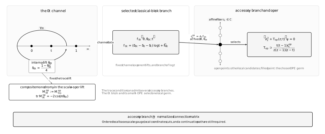
The internal channel fixes the lifted composite trace. A chosen small-$t$ block germ then selects an accessory branch through $c_t=\partial_tf_{0t}$ and therefore fixes the oper. This coefficient is not yet a normalized connection matrix: endpoint bases, scalar gauge, cuts, and a continuation path remain to be specified.

The block is a local generating function

At fixed external weights, the pairs $(t,c_t)$ serve as local Darboux coordinates on the four-puncture oper chart. A complementary monodromy chart uses the composite exponent $\theta_{0t}$ and a conjugate twist coordinate $\mu_{0t}$. In a chosen normalization, introduce

$$W(\theta_{0t},t) = W_0(\theta_{0t}) +f_{0t}(\theta_{0t},t),$$

where $W_0$ is independent of $t$. Locally,

$$\dd W = c_t\,\dd t +\mu_{0t}\,\dd\theta_{0t},$$

and hence

$$c_t = \partial_tW = \partial_tf_{0t}, \qquad \mu_{0t} = \partial_{\theta_{0t}}W.$$

This is the precise sense in which the block is a generating function. The $t$-independent term $W_0$ does not change the oper residue, but it does change the conjugate twist coordinate. Three-point chiral-vertex normalizations and branch changes that add a $t$-independent function live in this freedom. Changing an exponent representative is separate and may change $f_{0t}$ itself, hence the selected accessory branch.

Equivalently, in this convention the symplectic forms agree:

$$\dd c_t\wedge\dd t = \dd\theta_{0t}\wedge\dd\mu_{0t}.$$

This statement is local on a branch. It does not assert that one generating function covers the full character variety or survives every braid without a canonical transformation.

The standard Heun parameter is an affine transform

The normal residue $c_t$ is not the standard general-Heun parameter. Write the house Heun equation as

$$\begin{aligned} y''(z) &+ \left( \frac{\gamma_{\mathrm H}}z + \frac{\delta_{\mathrm H}}{z-1} + \frac{\epsilon_{\mathrm H}}{z-t} \right)y'(z) \\ &+ \frac{ \alpha_{\mathrm H}\beta_{\mathrm H}z-q_{\mathrm H} }{ z(z-1)(z-t) }y(z) =0. \end{aligned}$$

Choose one sign lift of each exponent difference and set

$$\begin{aligned} \gamma_{\mathrm H}&=1-\theta_0, & \delta_{\mathrm H}&=1-\theta_1, & \epsilon_{\mathrm H}&=1-\theta_t, \\ \alpha_{\mathrm H} &= 1-\frac{ \theta_0+\theta_1+\theta_t-\theta_\infty }{2}, \\ \beta_{\mathrm H} &= 1-\frac{ \theta_0+\theta_1+\theta_t+\theta_\infty }{2}. \end{aligned}$$

Then

$$\gamma_{\mathrm H} +\delta_{\mathrm H} +\epsilon_{\mathrm H} = \alpha_{\mathrm H} +\beta_{\mathrm H} +1,$$

and $\alpha_{\mathrm H}-\beta_{\mathrm H}=\theta_\infty$. On a simply connected patch, the scalar gauge is

$$\begin{aligned} y(z) ={}& z^{-\gamma_{\mathrm H}/2} (1-z)^{-\delta_{\mathrm H}/2} \left( 1-\frac zt \right)^{-\epsilon_{\mathrm H}/2} \psi(z). \end{aligned}$$

Define the shifted Heun coordinate

$$\kappa_{\mathrm H} := q_{\mathrm H} -\frac{\gamma_{\mathrm H}}2 \left( t\delta_{\mathrm H} +\epsilon_{\mathrm H} \right).$$

Direct substitution gives

$$c_t = \frac{ t\Lambda-\kappa_{\mathrm H} }{ t(t-1) }.$$

Therefore the exact CFT-to-Heun crosswalk is

$$\begin{aligned} q_{\mathrm H} ={}& \frac{\gamma_{\mathrm H}}2 \left( t\delta_{\mathrm H} +\epsilon_{\mathrm H} \right) +t\Lambda \\ &- t(t-1)\partial_tf_{0t}. \end{aligned}$$

For the unit-leading block this becomes

$$\begin{aligned} q_{\mathrm H} ={}& \frac{\gamma_{\mathrm H}}2 \left( t\delta_{\mathrm H} +\epsilon_{\mathrm H} \right) +t\Lambda \\ &- (t-1)\kappa_{\mathrm{OPE}} -t(t-1)\partial_t\widehat f_{0t}. \end{aligned}$$

Two differential checks catch the most common sign error. With $D(z)=z(z-1)(z-t)$,

$$\frac{\partial q_{\mathrm H}}{\partial c_t} = -t(t-1), \qquad \frac{\partial T_{\mathrm{op}}}{\partial q_{\mathrm H}} = -\frac1{D(z)}.$$

Changing a sign lift $\theta_i\mapsto-\theta_i$ changes the scalar gauge and performs a Heun index transformation. The normal-form double pole is unchanged, but the displayed Heun parameters—and generally $q_{\mathrm H}$—must be recomputed. Swapping $\alpha_{\mathrm H}$ and $\beta_{\mathrm H}$ alone leaves the equation unchanged.

The holomorphic block is not the uniformizing action

Two derivative formulae that look alike solve different problems.

Function	Defining data	What its derivative selects
$f_{0t}(t)$	A holomorphic chiral block, channel, internal weight, and analytic branch	A complex oper with prescribed lifted composite monodromy
$W_0+f_{0t}$	The same block plus a normalization-dependent, $t$-independent term	A local canonical transformation including the conjugate twist
Classical Liouville action $S_{\mathrm L}(t,\bar t)$	A full saddle, reality conditions, source data, and a regularization convention	The accessory data of a selected uniformizing or real-monodromy problem

The Polyakov relation for $S_{\mathrm L}$ carries convention-dependent signs and factors because some sources write the scalar equation with $T/2$. It should not be imported into $c_t=\partial_tf_{0t}$ by symbol matching. A full Liouville correlator also contains structure constants, an antiholomorphic block, an internal-momentum integral or sum, and possibly several saddles. Only after those ingredients are supplied can a saddle select a real or uniformizing solution.

What the classical block determines

Once the external weights and exponent lifts, $t$, the $0t$ channel and internal lift $\theta_{0t}$, the analytic block branch, and the full-block normalization are fixed, $\partial_tf_{0t}$ determines:

• the three constrained finite residues $c_0,c_t,c_1$;
• the complete four-pole normal-form coefficient $T_{\mathrm{op}}(z;t)$;
• the standard Heun parameter $q_{\mathrm H}$ after the declared scalar gauge;
• an oper whose selected composite monodromy has the internal-channel conjugacy class.

It does not directly determine:

• unit-leading Frobenius bases and their logarithmic or resonant limits;
• cuts, continuation paths, or determinant-one lift conventions;
• a normalized connection matrix between two local bases;
• finite degenerate fusion and braiding factors;
• the $t$-independent term $W_0$ or other three-point normalization data;
• the uniformizing Liouville saddle or a full CFT correlator.

The distinction is subtle but concrete. Fixing $T_{\mathrm{op}}$ fixes the differential equation, so its connection data can subsequently be computed. But a numerical connection matrix is defined only after both endpoint bases have been normalized. Classical-block derivatives provide the coefficient problem, not those two basis normalizations.

Common pitfalls

Writing $q_{\mathrm H}=\partial_tf_{0t}$. The derivative is the normal-form residue $c_t$. The standard Heun parameter differs by a gauge-dependent affine transformation.

Using a hatted block without the OPE pole. Removing the leading $t$-power shifts the classical derivative by $\kappa_{\mathrm{OPE}}/t$. The oper itself does not know that the notation was changed.

Treating the internal weight as all monodromy data. It fixes one composite conjugacy class, with a chosen lift and channel marking. A four-puncture character-variety point contains additional twist data.

Identifying a chiral block with the Liouville action. The former is holomorphic and channel-dependent. The latter belongs to a full saddle problem with reality, regularization, and antiholomorphic data.

Forgetting the scalar gauge. Normal and standard Heun forms have the same projective equation locally, but their exponent representatives and normalized bases differ by a generally multivalued factor.

Reading a connection matrix from one derivative. The accessory derivative fixes the ODE coefficient. Connection coefficients additionally require local basis normalizations and analytic continuation.

Exercises

1. Recover the constrained residues

Starting from the two conditions at infinity, solve for $c_0$ and $c_1$ in terms of $c_t$ and $\Lambda$.

Solution

The first condition gives $c_0=-c_t-c_1$. The second gives

$$tc_t+c_1=\Lambda,$$

so

$$c_1=\Lambda-tc_t.$$

Substitution into the first condition yields

$$c_0=-\Lambda+(t-1)c_t.$$

Partial-fraction recombination then gives the compact oper displayed on this page.

2. Restore the OPE-prefactor contribution

Suppose a computation returns $\partial_t\widehat f_{0t}$. Express the full oper residue in terms of that result.

Solution

The two classical blocks differ by

$$f_{0t} = \kappa_{\mathrm{OPE}}\Log t +\widehat f_{0t}.$$

Therefore

$$c_t = \partial_tf_{0t} = \frac{\kappa_{\mathrm{OPE}}}{t} +\partial_t\widehat f_{0t}.$$

The branch of $\Log t$ changes $f_{0t}$ by a constant but does not change this local derivative away from $t=0$.

3. Derive the Heun crosswalk

Use $c_t=(t\Lambda-\kappa_{\mathrm H})/[t(t-1)]$ and the definition of $\kappa_{\mathrm H}$ to solve for $q_{\mathrm H}$.

Solution

First,

$$\kappa_{\mathrm H} = t\Lambda -t(t-1)c_t.$$

Since

$$\kappa_{\mathrm H} = q_{\mathrm H} -\frac{\gamma_{\mathrm H}}2 \left( t\delta_{\mathrm H} +\epsilon_{\mathrm H} \right),$$

one obtains

$$\begin{aligned} q_{\mathrm H} ={}& \frac{\gamma_{\mathrm H}}2 \left( t\delta_{\mathrm H} +\epsilon_{\mathrm H} \right) +t\Lambda \\ &- t(t-1)c_t. \end{aligned}$$

Substituting $c_t=\partial_tf_{0t}$ gives the CFT formula.

4. Recover the composite trace

In the sewing annulus, the effective fused $0t$ channel has normal-form powers $(1\pm\theta_{0t})/2$. Show that they give the displayed trace of $M_{0t}$.

Solution

Continuation of these effective fused-channel branches once counterclockwise multiplies them by

$$\exp \left[ 2\pi\ii \frac{1\pm\theta_{0t}}2 \right] = -\ee^{\pm\pi\ii\theta_{0t}}.$$

Their sum is

$$\operatorname{tr}M_{0t} = -2\cos(\pi\theta_{0t}).$$

This calculation fixes a determinant-one scalar-oper lift. Multiplying the monodromy by the central matrix $-I$ reverses the sign of the trace without changing projective monodromy.

5. Add a modulus-independent classical normalization

Let $\widetilde f=f+A(\theta_{0t})$. Which quantities on this page change?

Solution

Because $A$ is independent of $t$,

$$\partial_t\widetilde f = \partial_tf.$$

Therefore $c_t$, the oper, and $q_{\mathrm H}$ do not change. By contrast,

$$\partial_{\theta_{0t}}\widetilde f = \partial_{\theta_{0t}}f +A'(\theta_{0t}),$$

so the conjugate twist coordinate changes. This is why three-point or chiral-vertex normalizations can be invisible to the accessory residue but visible to normalized connection data.

6. Turn sewing data into an accessory series

Given $\widehat f_{0t}=\kappa_1t+\kappa_2t^2+O(t^3)$, find $c_t$ and the constant term of $q_{\mathrm H}$ as $t\to0$.

Solution

Differentiation gives

$$c_t = \frac{\kappa_{\mathrm{OPE}}}{t} +\kappa_1 +2\kappa_2t +O(t^2).$$

Insert this into the Heun crosswalk. Since $-t(t-1)c_t\to\kappa_{\mathrm{OPE}}$,

$$q_{\mathrm H}(t) = \frac{ \gamma_{\mathrm H}\epsilon_{\mathrm H} }{2} +\kappa_{\mathrm{OPE}} +O(t).$$

Equivalently, the constant term is

$$q_{\mathrm H}(0) = \frac{ (1-\theta_0-\theta_t)^2-\theta_{0t}^2 }{4}.$$

The finite limit concerns the chosen Heun coordinate; the four-puncture geometry itself degenerates at $t=0$.

7. Change the endpoint basis normalizations

Suppose two fundamental matrices obey $\Phi_b=\Phi_aC_{ab}$. If the local bases are rescaled as $\Phi_a\mapsto\Phi_aD_a$ and $\Phi_b\mapsto\Phi_bD_b$, determine the new connection matrix.

Solution

Write

$$\Phi_bD_b = \Phi_aD_a\,\widetilde C_{ab}.$$

Using $\Phi_b=\Phi_aC_{ab}$ gives

$$\widetilde C_{ab} = D_a^{-1}C_{ab}D_b.$$

The oper coefficient is unchanged, but the numerical connection matrix changes. An accessory derivative therefore cannot specify a normalized connection matrix until $D_a$ and $D_b$ have been fixed.

References

• A. Litvinov, S. Lukyanov, N. Nekrasov, and A. Zamolodchikov, “Classical Conformal Blocks and Painlevé VI”, Journal of High Energy Physics 2014 (2014), 144. Equations (2.1), (2.9), and (2.13)–(2.14) give the oper, accessory gradient, and four-point specialization; the internal channel fixes composite monodromy traces.
• J. Teschner, “Classical Conformal Blocks and Isomonodromic Deformations”, 2017. Develops classical blocks as generating functions on moduli spaces of flat connections and relates their branches to isomonodromic geometry.
• N. Nekrasov, A. Rosly, and S. Shatashvili, “Darboux Coordinates, Yang–Yang Functional, and Gauge Theory”, Nuclear Physics B Proceedings Supplements 216 (2011), 69–93. Supplies the Darboux-coordinate and generating-function interpretation.
• G. Bonelli, C. Iossa, D. Panea Lichtig, and A. Tanzini, “Irregular Liouville Correlators and Connection Formulae for Heun Functions”, Communications in Mathematical Physics 397 (2023), 635–727. Gives normalization-aware BPZ-to-Heun dictionaries and displays the finite factors not captured by an accessory derivative alone.
• M. Piątek and A. R. Pietrykowski, “Solving Heun’s Equation Using Conformal Blocks”, Nuclear Physics B 938 (2019), 543–570. Provides an independent standard-to-normal-form Heun convention check and derives Floquet-type solutions from degenerate classical blocks.
• L. A. Takhtajan and P. G. Zograf, “Hyperbolic 2-Spheres with Conical Singularities, Accessory Parameters and Kähler Metrics on $\mathcal M_{0,n}$”, Transactions of the American Mathematical Society 355 (2003), 1857–1867. Relates the classical Liouville action to the distinct Fuchsian uniformization problem; its scalar-equation normalization differs from the one used here.
• NIST Digital Library of Mathematical Functions, §31.2, Heun equations and §31.14, Fuchsian equations, for the canonical general-Heun equation and accessory-parameter count.