Hamiltonian Structure and Accessory Parameters

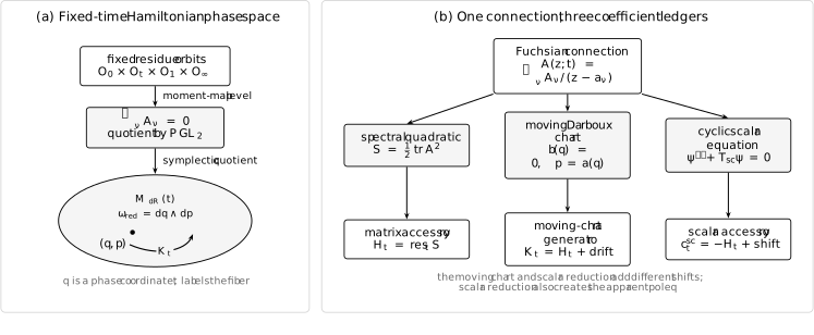
Three nearby quantities are easily conflated: the residue Hamiltonian $H_i$, the moving-chart Hamiltonian $K_t$, and the scalar accessory residue $c_i^{\mathrm{sc}}$. The apparent-pole position $q$ is a coordinate, not a fourth accessory parameter. On the residue-orbit phase space, the generator is

$$H_i = \sum_{j\ne i} \frac{\operatorname{tr}(A_iA_j)}{a_i-a_j}.$$

The same function is the simple-pole residue of $\tfrac12\operatorname{tr}A(z)^2$. This book therefore calls it a spectral or matrix accessory, while reserving “scalar accessory” for a coefficient of a scalar normal equation. After passing to an explicitly time-dependent Darboux chart, the canonical Hamiltonian acquires a correction. After scalar projection, the accessory coefficient acquires a different cyclic-vector and gauge correction.

This page derives the three dictionaries without identifying their entries:

Object	Definition	Role
$H_i$	$\operatorname*{res}_{z=a_i}\tfrac12\operatorname{tr}A(z)^2$	Schlesinger generator in residue variables and matrix accessory
$K_t$	$H_t$ plus the moving-chart correction	Canonical generator for the declared $(q,p)$ coordinates
$c_i^{\mathrm{sc}}$	Simple-pole residue of the scalar projective connection	Scalar normal-form accessory after choosing a cyclic vector
$q$	Zero of $A_{12}(z)$	Darboux position and apparent scalar pole, not the Heun accessory $q_{\mathrm H}$

First pass

Read the KKS sign calculation, check that $H_i$ reproduces Schlesinger, follow the quadratic-differential expansion, and compare $H_t$, $K_t$, and $c_t^{\mathrm{sc}}$ in the exact benchmark. The time-dependent canonical transformation and polynomial Painlevé convention can be postponed.

Residue orbits carry the phase-space symplectic form

Fix the finite pole positions and the adjoint orbits $\mathcal O_i$ of the residues. An adjoint orbit fixes a residue’s eigenvalues while allowing its eigendirections to vary. The unreduced space used for the Hamiltonian calculation is

$$\mathcal P = \prod_{i=1}^{n}\mathcal O_i.$$

We now fix the overall sign left open on the chapter’s first page. If

$$\delta_1A_i=[X_i,A_i], \qquad \delta_2A_i=[Y_i,A_i],$$

then

$$\omega_{\mathcal P} (\delta_1A,\delta_2A) = \sum_{i=1}^{n} \operatorname{tr} \left( A_i[X_i,Y_i] \right),$$

This is the Kirillov–Kostant–Souriau (KKS) form in the declared trace-pairing convention.

and Hamiltonian vector fields are defined by

$$\iota_{X_F}\omega_{\mathcal P}=\dd F.$$

Use the trace pairing to define gradients:

$$\dd F(\delta A) = \sum_i \operatorname{tr} \left( \nabla_iF\,\delta A_i \right).$$

For a tangent vector $\delta A_i=[X_i,A_i]$,

$$\dd F(\delta A) = \sum_i \operatorname{tr} \left( [A_i,\nabla_iF]X_i \right).$$

Comparing with the KKS form gives

$$X_F(A_i)=[\nabla_iF,A_i].$$

Equivalently, the Lie–Poisson bracket is

$$\{F,G\} = \sum_i \operatorname{tr} \left( A_i[\nabla_iF,\nabla_iG] \right),$$

and evolution generated by $H$ obeys

$$\frac{\dd F}{\dd s}=\{F,H\}.$$

This convention is sign-sensitive. Some references combine the opposite KKS sign with $\iota_{X_H}\omega=-\dd H$. Either complete convention is consistent; mixing one half of each reverses the Schlesinger flow.

The additive moment map and reduction

Simultaneous conjugation acts by

$$A_i\longmapsto GA_iG^{-1}.$$

To impose the residue theorem while fixing the orbit at infinity, enlarge the product to

$$\mathcal P_{\mathrm{ext}} = \mathcal O_1\times\cdots\times \mathcal O_n\times\mathcal O_\infty.$$

For $X\in\mathfrak{sl}_2$, the function

$$\mu_X = \operatorname{tr} \left( X\sum_{\nu\in\{1,\ldots,n,\infty\}}A_\nu \right)$$

generates $\delta A_i=[X,A_i]$. Thus the moment map is

$$\mu_{\mathrm{add}}=\sum_iA_i.$$

In these two moment-map formulas, the sum includes the infinity residue. Reduction at zero imposes the residue theorem and removes the common basis:

$$\left( \mathcal O_1\times\cdots\times\mathcal O_\infty \right) \mathbin{//}PGL(2,\mathbb C).$$

Four generic $\mathfrak{sl}_2$ orbits contribute eight complex dimensions. The three moment-map equations and the three-dimensional conjugation quotient leave a complex surface. This is the fixed-$t$ phase space from the chapter overview.

The dimension count assumes a transverse moment-map level and a locally free effective action. Reducible tuples and central orbits can make the quotient singular even though the matrix differential equations remain meaningful.

The Schlesinger equations are Hamilton’s equations

For one finite pole $a_r$, define

$$H_r = \sum_{j\ne r} \frac{\operatorname{tr}(A_rA_j)} {a_r-a_j}.$$

The gradients are immediate:

$$\begin{aligned} \nabla_jH_r &= \frac{A_r}{a_r-a_j}, &&j\ne r, \\ \nabla_rH_r &= \sum_{j\ne r} \frac{A_j}{a_r-a_j}. \end{aligned}$$

Therefore, for $j\ne r$,

$$X_{H_r}(A_j) = \frac{[A_r,A_j]}{a_r-a_j},$$

while

$$X_{H_r}(A_r) = -\sum_{j\ne r} \frac{[A_r,A_j]}{a_r-a_j}.$$

These are exactly the off-diagonal and diagonal Schlesinger equations from the preceding page:

$$\frac{\partial A_j}{\partial a_r} = X_{H_r}(A_j).$$

Each $H_r$ is invariant under simultaneous conjugation, preserves the moment-map level, and descends to the reduced phase space. The family is nonautonomous: its denominators contain the pole positions explicitly. Consequently $H_r$ is generally not a conserved energy along its own time:

$$\frac{\dd H_r}{\dd a_r} = \frac{\partial H_r}{\partial a_r}.$$

The rational Gaudin identities

$$\{H_r,H_s\}=0, \qquad \frac{\partial H_r}{\partial a_s} = \frac{\partial H_s}{\partial a_r}$$

encode multi-time compatibility. Their combination will become the closedness calculation for the tau-function one-form on the next page.

A spectral quadratic differential exposes the accessories

Set

$$\mathcal S(z) = \frac12\operatorname{tr}A(z)^2, \qquad \Delta_i = \frac12\operatorname{tr}(A_i^2).$$

For traceless rank two with residue eigenvalues $\pm\theta_i/2$,

$$\Delta_i=\frac{\theta_i^2}{4}.$$

Partial fractions give the exact identity

$$\mathcal S(z) = \sum_{i=1}^{n} \left[ \frac{\Delta_i}{(z-a_i)^2} + \frac{H_i}{z-a_i} \right].$$

Indeed, the cross term involving $A_i$ and $A_j$ contributes

$$\frac{\operatorname{tr}(A_iA_j)} {(z-a_i)(z-a_j)},$$

whose residue at $a_i$ is $\operatorname{tr}(A_iA_j)/(a_i-a_j)$. Thus the Schlesinger Hamiltonian is literally a simple-pole coefficient of the conjugation-invariant quadratic differential $\mathcal S(z)\,\dd z^2$.

Expanding at infinity gives two constraints:

$$\sum_iH_i=0,$$

and

$$\sum_i \left( \Delta_i+a_iH_i \right) = \Delta_\infty, \qquad \Delta_\infty = \frac12\operatorname{tr}(A_\infty^2).$$

There are therefore $n-2$ independent matrix accessories among the $n$ finite $H_i$, matching the number of true deformation times. This mirrors the scalar accessory count in Chapter 3, but the coefficients are not yet the scalar normal-form residues.

One matrix accessory for four poles

For poles $0,t,1,\infty$, write

$$\Lambda = \Delta_\infty-\Delta_0-\Delta_t-\Delta_1.$$

Then

$$\begin{aligned} \mathcal S(z) ={}& \frac{\Delta_0}{z^2} + \frac{\Delta_t}{(z-t)^2} + \frac{\Delta_1}{(z-1)^2} \\ &+ \frac{\Lambda}{z(z-1)} + \frac{t(t-1)H_t} {z(z-1)(z-t)}. \end{aligned}$$

The other two finite residues are

$$H_0=(t-1)H_t-\Lambda, \qquad H_1=\Lambda-tH_t.$$

This is the matrix analogue of the four-point projective-connection formula. The double-pole coefficients differ already: $\Delta_i=\theta_i^2/4$ here, whereas the scalar normal equation uses $(1-\theta_i^2)/4$.

One residue tuple produces three related but distinct coefficients. $H_t$ is the spectral residue and residue-coordinate Hamiltonian; $K_t$ generates motion in the explicitly time-dependent Darboux chart; scalar projection produces $c_t^{\mathrm{sc}}$ and a moving apparent pole $q$.

A zero of the off-diagonal entry is a Darboux coordinate

On the open set where $A_\infty$ is regular semisimple, so $\theta_\infty\ne0$, fix its eigenline ordering by choosing

$$A_\infty = \begin{pmatrix} \theta_\infty/2&0\\ 0&-\theta_\infty/2 \end{pmatrix},$$

and write

$$A(z) = \begin{pmatrix} a(z)&b(z)\\ c(z)&-a(z) \end{pmatrix}.$$

Here $a(z)$ denotes the diagonal matrix entry; it is unrelated to the pole labels $a_i$.

Since the upper-right entry of $A_\infty$ vanishes, the finite upper-right residues sum to zero. On the open set where $b$ is not identically zero and has one simple finite zero away from the true poles,

$$b(z) = \frac{\chi(z-q)} {z(z-1)(z-t)}, \qquad \chi\ne0.$$

The harmless minus sign used for this formula in the chapter overview has been absorbed into the nonzero scale $\chi$.

Define

$$p=a(q).$$

The residual diagonal conjugation preserving $A_\infty$ rescales $\chi$ but fixes $q$ and $p$, so both descend to the quotient.

To prove that they are canonical, the matrix-entry Poisson bracket is more efficient than a residue parametrization. If $b_i=(A_i)_{12}$ and $h_i=(A_i)_{11}$, the KKS convention gives

$$\{b_i,h_j\} = \delta_{ij}b_i.$$

Summing over the finite poles, or equivalently computing with invariant local extensions before reduction, gives

$$\{b(z),a(w)\} = \frac{b(z)-b(w)}{w-z}.$$

The root variables are invariant under the residual diagonal stabilizer, so this is also the induced bracket on the gauge-fixed quotient.

Differentiate the identity $b(q)=0$ by taking its bracket with $a(w)$:

$$0 = -\frac{b(w)}{w-q} + b'(q)\{q,a(w)\}.$$

Hence

$$\{q,a(w)\} = \frac{b(w)} {(w-q)b'(q)}.$$

Taking $w\to q$ gives

$$\{q,p\}=1, \qquad \omega_{\mathrm{red}}=\dd q\wedge\dd p$$

in the declared convention. The composition $p=a(q)$ introduces no extra chain term because $\{q,q\}=0$.

At the zero of $b$, the matrix $A(q)$ is triangular and

$$\mathcal S(q)=a(q)^2=p^2.$$

Substituting the four-pole expression for $\mathcal S$ and solving for $H_t$ yields

$$\begin{aligned} H_t ={}& \frac{q(q-1)(q-t)} {t(t-1)} \Biggl[ p^2 - \frac{\Delta_0}{q^2} - \frac{\Delta_1}{(q-1)^2} \\ &\hspace{5.2em} - \frac{\Delta_t}{(q-t)^2} - \frac{\Lambda}{q(q-1)} \Biggr]. \end{aligned}$$

This is the bare spectral accessory expressed in fixed-time Darboux coordinates. It is not yet the Hamiltonian that differentiates those coordinates while $t$ moves.

The moving Darboux chart shifts the Hamiltonian

The definition of $q$ contains the moving pole $t$. Even if the residue matrices were frozen, changing $t$ would change the zero of $b(z)$. That explicit coordinate drift must be added to the Hamiltonian vector field.

Differentiate $b(q,t)=0$ along the Lax system:

$$0 = \left( \frac{\partial b}{\partial t} \right)(q,t) + b'(q,t)\dot q.$$

At $z=q$,

$$\left. \frac{\partial b}{\partial t} \right|_{z=q} = \frac{(A_t)_{12}}{(q-t)^2} + \frac{2p(A_t)_{12}}{q-t},$$

whereas the rational form of $b$ gives

$$\frac{(A_t)_{12}}{b'(q)} = -\frac{ q(q-1)(q-t)^2 }{ t(t-1) }.$$

Therefore

$$\frac{\dd q}{\dd t} = \frac{q(q-1)} {t(t-1)} \left[ 2(q-t)p+1 \right].$$

The $p$-derivative of the bare $H_t$ supplies only the term proportional to $2(q-t)p$. A direct calculation of the explicit drift of $p=a(q)$, using

$$a(z) = -\frac{\theta_\infty}{2z} + O(z^{-2}) \qquad (z\to\infty),$$

gives

$$\begin{aligned} \dot p &= \left( \frac{\partial a}{\partial t} \right)(q,t) + a'(q,t)\dot q \\ &= -\frac{\partial H_t}{\partial q} - \frac{(2q-1)p}{t(t-1)} - \frac{\theta_\infty}{2t(t-1)}. \end{aligned}$$

This fixes the remaining $q$-dependent term. The canonical equations

$$\frac{\dd q}{\dd t} = \frac{\partial K_t}{\partial p}, \qquad \frac{\dd p}{\dd t} = -\frac{\partial K_t}{\partial q}$$

hold for

$$K_t = H_t + \frac{q(q-1)p}{t(t-1)} + \frac{\theta_\infty q}{2t(t-1)} + f(t).$$

The arbitrary $f(t)$ does not change Hamilton’s equations. The JMU convention on the next page fixes $\partial_t\log\tau=H_t$. Thus $f(t)$ is dynamically invisible but must be retained when comparing $K_t$ with a tau derivative: it changes the corresponding representative by $\exp[\int f(t)\,\dd t]$, not merely by the standard constant ambiguity.

The distinction is structural:

• $H_t$ is invariantly defined in the residue chart and is the simple residue of $\mathcal S$;
• $K_t$ generates the same flow after the phase coordinates themselves have been made explicitly time-dependent;
• a different time-dependent canonical chart adds the derivative of its generating function.

Swapping the two eigenlines at infinity changes the sign of the $\theta_\infty$-linear correction. Squared local spectral data alone do not remember that ordering.

One polynomial Painlevé convention

Define a shifted momentum

$$P = p + \frac12 \left[ \frac{\theta_0}{q} + \frac{\theta_1}{q-1} + \frac{\theta_t}{q-t} \right].$$

The change is time-dependent. A generating function is

$$F_{\mathrm{gen}} = -\frac12 \left[ \theta_0\log q + \theta_1\log(q-1) + \theta_t\log(q-t) \right],$$

so the new Hamiltonian also receives $\partial_tF_{\mathrm{gen}}=\theta_t/[2(q-t)]$. Up to a function of $t$,

$$\begin{aligned} t(t-1)K_{\mathrm{VI}} ={}& q(q-1)(q-t)P^2 \\ &- \Bigl[ \theta_0(q-1)(q-t) + \theta_1q(q-t) \\ &\hspace{3.0em} + (\theta_t-1)q(q-1) \Bigr]P \\ &+ \kappa(q-t), \end{aligned}$$

where

$$\kappa = \frac{ (\theta_0+\theta_1+\theta_t-1)^2 - (\theta_\infty-1)^2 }{4}.$$

This is one standard polynomial normalization. Other momenta, eigenline orderings, and contraction signs change its appearance. The later Painlevé–Heun page eliminates $P$ and fixes its own parameter dictionary.

Scalar projection shifts every accessory residue

The spectral quadratic differential $\mathcal S$ is not the scalar projective connection from Chapter 3. Eliminate the second component of $Y$ where $b\ne0$. The first component $y$ obeys

$$y'' - \frac{b'}b\,y' - \left( a'+\mathcal S-a\frac{b'}b \right)y =0.$$

Set $y=\sqrt b\,\psi$. Then

$$\psi''+T_{\mathrm{sc}}(z)\psi=0,$$

with

$$\begin{aligned} T_{\mathrm{sc}} ={}& -\mathcal S-a' + a\frac{b'}b \\ &+ \frac12 \left( \frac{b'}b \right)' - \frac14 \left( \frac{b'}b \right)^2. \end{aligned}$$

Near a true finite pole $a_i$, write

$$\begin{aligned} a(z) &= \frac{h_i}{z-a_i} + a_i^{\mathrm{reg}} + O(z-a_i), \\ \frac{b'}b &= -\frac1{z-a_i} + \ell_i + O(z-a_i). \end{aligned}$$

The double-pole coefficient becomes

$$\frac{1-\theta_i^2}{4},$$

as required for scalar exponent difference $\theta_i$. The simple-pole coefficient is

$$c_i^{\mathrm{sc}} = -H_i - a_i^{\mathrm{reg}} + \left( h_i+\frac12 \right)\ell_i.$$

For the four-pole rational form,

$$\begin{aligned} a_i^{\mathrm{reg}} &= \sum_{j\ne i} \frac{h_j}{a_i-a_j}, \\ \ell_i &= \frac1{a_i-q} - \sum_{j\ne i} \frac1{a_i-a_j}. \end{aligned}$$

Thus even the sign-adjusted guess $c_i^{\mathrm{sc}}=-H_i$ misses explicit cyclic-vector and scalar-gauge terms.

At the zero $q$ of $b$, the scalar coefficient has

$$T_{\mathrm{sc}}(z) = -\frac{3}{4(z-q)^2} + \frac{c_q}{z-q} + O(1),$$

where

$$c_q = p + \frac12 \sum_{j\in\{0,t,1\}} \frac1{q-a_j}.$$

The local exponents are $-1/2$ and $3/2$. Because both scalar solutions come from a regular matrix system at $q$, the singularity is apparent. If the regular term is $d_q+O(z-q)$, the no-log condition is

$$d_q=-c_q^2.$$

A generic cyclic reduction therefore has the four true singularities plus the apparent pole $q$. It is not the four-singularity Heun equation of Chapter 3. Removing or constraining the apparent pole requires an additional specialization or tau/accessory relation developed on the Painlevé–Heun page.

An exact irreducible checkpoint

At $t=2$, take

$$A_0 = \begin{pmatrix} \tfrac12&1\\ 1&-\tfrac12 \end{pmatrix}, \qquad A_t = \begin{pmatrix} -\tfrac13&2\\ 2&\tfrac13 \end{pmatrix},$$

and

$$A_1 = \begin{pmatrix} \tfrac14&-3\\ -3&-\tfrac14 \end{pmatrix}, \qquad A_\infty = \begin{pmatrix} -\tfrac5{12}&0\\ 0&\tfrac5{12} \end{pmatrix}.$$

The four residues sum to zero. Moreover,

$$\det[A_t,A_0]=\frac{64}{9}\ne0,$$

so $A_0$ and $A_t$ are not simultaneously triangularizable; the tuple is irreducible. All four exponent differences are nonintegral.

The upper-right entry is

$$b(z) = \frac1z+\frac2{z-2}-\frac3{z-1} = \frac{z+2}{z(z-1)(z-2)}.$$

Hence

$$q=-2, \qquad p=a(q)=-\frac14.$$

The spectral invariants are

$$\left( \Delta_0,\Delta_t,\Delta_1,\Delta_\infty \right) = \left( \frac54,\frac{37}{9},\frac{145}{16},\frac{25}{144} \right).$$

Direct traces, or the identity $\mathcal S(q)=p^2$, give

$$H_t=-\frac{31}{3}.$$

The chosen infinity ordering has $\theta_\infty=-5/6$, so the moving-coordinate formula gives

$$K_t\big|_{f=0} = -\frac{32}{3}, \qquad \dot q = \frac{\partial K_t}{\partial p} =9.$$

This checks the momentum-linear drift. The other Hamilton equation also tests the sign of the $\theta_\infty$ correction. Direct Schlesinger differentiation gives

$$\left( \frac{\partial a}{\partial t} \right)(q) = -\frac1{48}, \qquad a'(q)=-\frac{19}{144},$$

and therefore

$$\dot p = -\frac1{48} - \frac{19}{144}\,9 = -\frac{29}{24} = -\frac{\partial K_t}{\partial q}.$$

For the scalar residue at $t=2$,

$$h_t=-\frac13, \qquad a_t^{\mathrm{reg}}=\frac12, \qquad \ell_t=-\frac54.$$

Therefore

$$c_t^{\mathrm{sc}} = -H_t-a_t^{\mathrm{reg}} + \left( h_t+\frac12 \right)\ell_t = \frac{77}{8}.$$

The three numbers

$$H_t=-\frac{31}{3}, \qquad K_t\big|_{f=0}=-\frac{32}{3}, \qquad c_t^{\mathrm{sc}}=\frac{77}{8}$$

are deliberately unequal. They describe one connection in three coordinate constructions. As a further exact check,

$$c_q=-\frac{19}{24}.$$

The initial tuple determines a unique local Schlesinger trajectory, so these identities are not confined to a static algebra exercise.

Where the coordinate dictionaries can fail

Darboux-chart boundary. The declared $(q,p)$ chart requires $b\not\equiv0$, a simple finite zero $q$, and $q\notin\{0,t,1,\infty\}$. At a failure, choose the other component or an adjacent Okamoto chart; the abstract phase point need not be singular.

Singular quotient. At reducible tuples the stabilizer jumps, so a coarse quotient can be singular. The KKS equations on the unreduced product still make algebraic sense.

Gauge dependence. A $z$-independent simultaneous conjugation preserves $\mathcal S$ and $H_i$. A meromorphic $z$-dependent gauge changes $A$ by an inhomogeneous derivative term and need not preserve the printed coefficients.

Canonical-convention dependence. Momentum shifts, eigenline swaps, and time-dependent generating functions change the displayed Hamiltonian. They do not change the underlying isomonodromic leaf when transformed consistently.

Collision versus chart failure. The fixed times $t=0,1,\infty$ are pole collisions. A finite $q$ reaching a true pole is instead a failure of this Darboux chart. The two require different responses.

Common pitfalls

Treating $H_t$ as conserved energy. Schlesinger is a nonautonomous Hamiltonian system. The same $H_t$ will become a logarithmic tau derivative, not a constant of motion.

Using bare $H_t$ in moving $(q,p)$ coordinates. The zero defining $q$ depends explicitly on $t$. The correction from $H_t$ to $K_t$ is required before writing canonical time derivatives.

Equating matrix and scalar accessories. The scalar cyclic-vector reduction and Liouville transform contribute explicit shifts. Generic scalarization also introduces an apparent pole.

Calling the apparent coordinate the Heun accessory. This page uses $q$ for a moving apparent position. The standard Heun accessory is denoted $q_{\mathrm H}$ and belongs to a different parameter dictionary.

Treating one chart as the whole Painlevé surface. The rational $(q,p)$ coordinates cover a large open set, not every stable parabolic connection.

Exercises

1. Derive the Hamiltonian vector field

Starting with the KKS form and $\iota_{X_F}\omega=\dd F$, prove $X_F(A_i)=[\nabla_iF,A_i]$ and derive the Lie–Poisson bracket.

Solution

For $\delta A_i=[X_i,A_i]$,

$$\dd F(\delta A) = \sum_i \operatorname{tr} \left( [A_i,\nabla_iF]X_i \right).$$

If $X_F(A_i)=[K_i,A_i]$, then

$$\omega(X_F,\delta A) = \sum_i \operatorname{tr} \left( [A_i,K_i]X_i \right).$$

Thus $K_i=\nabla_iF$ modulo the centralizer of $A_i$, which does not alter the tangent vector. Evaluating $\dd F$ on $X_G$ gives

$$\{F,G\} = \sum_i \operatorname{tr} \left( A_i[\nabla_iF,\nabla_iG] \right).$$

2. Recover the four-pole Schlesinger flow

Use

$$H_t = \frac{\operatorname{tr}(A_tA_0)}t + \frac{\operatorname{tr}(A_tA_1)}{t-1}$$

to reproduce the equations for $A_0,A_t,A_1$.

Solution

The three gradients are

$$\nabla_0H_t=\frac{A_t}{t}, \qquad \nabla_1H_t=\frac{A_t}{t-1},$$

and

$$\nabla_tH_t = \frac{A_0}{t} + \frac{A_1}{t-1}.$$

Applying $X_H(A)=[\nabla H,A]$ gives

$$\dot A_0=\frac{[A_t,A_0]}t, \qquad \dot A_1=\frac{[A_t,A_1]}{t-1},$$

and

$$\dot A_t = -\frac{[A_t,A_0]}t - \frac{[A_t,A_1]}{t-1}.$$

3. Derive the accessory constraints at infinity

Expand the partial-fraction expression for $\mathcal S(z)$ at infinity and derive the two constraints on the $H_i$.

Solution

Using

$$\frac1{z-a_i} = \frac1z+\frac{a_i}{z^2}+O(z^{-3}), \qquad \frac1{(z-a_i)^2} = \frac1{z^2}+O(z^{-3}),$$

gives

$$\mathcal S(z) = \frac{\sum_iH_i}{z} + \frac{ \sum_i(\Delta_i+a_iH_i) }{z^2} + O(z^{-3}).$$

But $A(z)=-A_\infty/z+O(z^{-2})$, so

$$\mathcal S(z) = \frac{\Delta_\infty}{z^2} + O(z^{-3}).$$

Equating coefficients proves

$$\sum_iH_i=0, \qquad \sum_i(\Delta_i+a_iH_i)=\Delta_\infty.$$

4. Prove that q and p are canonical

Starting from the rational matrix-entry bracket and $b(q)=0$, prove $\{q,p\}=1$.

Solution

Taking the bracket of $b(q)=0$ with $a(w)$ gives

$$0 = \{b(z),a(w)\}_{z=q} + b'(q)\{q,a(w)\}.$$

Since $b(q)=0$,

$$\{b(z),a(w)\}_{z=q} = -\frac{b(w)}{w-q}.$$

Therefore

$$\{q,a(w)\} = \frac{b(w)} {(w-q)b'(q)}.$$

The limit $w\to q$ is one. Because $p=a(q)$ and $\{q,q\}=0$, it follows that $\{q,p\}=1$.

5. Find the moving-chart correction

Show first that the Lax equation gives

$$\dot q = \frac{q(q-1)} {t(t-1)} \left[ 2(q-t)p+1 \right].$$

Compare this with $\partial_pH_t$ and recover the term in $K_t$ that is linear in $p$. Then use the $p$-equation to recover the $\theta_\infty$-linear term.

Solution

Differentiate the root condition:

$$\dot q = -\frac{\partial_tb(q,t)}{b'(q,t)}.$$

The $(1,2)$ entry of the Lax equation and the residue of the rational $b(z)$ at $z=t$ give

$$\partial_tb(q,t) = \frac{(A_t)_{12}}{(q-t)^2} + \frac{2p(A_t)_{12}}{q-t},$$

and

$$\frac{(A_t)_{12}}{b'(q)} = -\frac{q(q-1)(q-t)^2}{t(t-1)}.$$

Combining them proves the displayed $\dot q$. Since

$$\partial_pH_t = \frac{2q(q-1)(q-t)p}{t(t-1)},$$

the missing term is generated by $q(q-1)p/[t(t-1)]$. The $p$-equation and the chosen infinity ordering fix the remaining correction. In fact,

$$\dot p+\partial_qH_t = -\frac{(2q-1)p}{t(t-1)} - \frac{\theta_\infty}{2t(t-1)}.$$

Integrating the right-hand side with respect to $-q$ yields

$$\frac{q(q-1)p}{t(t-1)} + \frac{\theta_\infty q}{2t(t-1)},$$

up to $f(t)$.

6. Derive the scalar accessory shift

Starting from the first-component equation, perform the Liouville transformation and recover $c_i^{\mathrm{sc}}$ at a true pole.

Solution

For an equation $y''+P y'+Qy=0$, the substitution $y=\exp[-\tfrac12\int P\,\dd z]\psi$ gives

$$\psi'' + \left( Q-\frac12P'-\frac14P^2 \right)\psi =0.$$

Here $P=-b'/b$ and $Q=-a'-\mathcal S+a\,b'/b$, producing the stated $T_{\mathrm{sc}}$.

Insert

$$a=\frac{h_i}{x}+a_i^{\mathrm{reg}}+O(x), \qquad \frac{b'}b=-\frac1x+\ell_i+O(x), \qquad x=z-a_i.$$

The $x^{-2}$ coefficient is $-\Delta_i+1/4=(1-\theta_i^2)/4$. The $x^{-1}$ coefficient is

$$-H_i-a_i^{\mathrm{reg}} + \left( h_i+\frac12 \right)\ell_i,$$

which is $c_i^{\mathrm{sc}}$.

7. Audit the irreducible rational tuple

For the matrices in the exact checkpoint, compute $q,p,H_t,K_t$, and $c_t^{\mathrm{sc}}$ independently. Verify both $\dot q$ and $\dot p$ from the Schlesinger equations.

Solution

The upper-right entry immediately gives $q=-2$, while substituting into the diagonal entry gives $p=-1/4$. Direct traces yield

$$H_t = \frac{\operatorname{tr}(A_tA_0)}2 + \operatorname{tr}(A_tA_1) = -\frac{31}{3}.$$

At $t=2$,

$$\frac{q(q-1)}{t(t-1)}=3, \qquad \theta_\infty=-\frac56.$$

Hence

$$K_t\big|_{f=0} = -\frac{31}{3} + 3\left(-\frac14\right) + \frac{(-5/6)(-2)}4 = -\frac{32}{3}.$$

For the two coordinate derivatives,

$$\dot q=9, \qquad \left( \frac{\partial a}{\partial t} \right)(q) = -\frac1{48}, \qquad a'(q)=-\frac{19}{144}.$$

Thus

$$\dot p = \left( \frac{\partial a}{\partial t} \right)(q) + a'(q)\dot q = -\frac{29}{24},$$

which agrees with $-\partial_qK_t$.

Finally,

$$c_t^{\mathrm{sc}} = \frac{31}{3} - \frac12 + \left( -\frac13+\frac12 \right) \left( -\frac54 \right) = \frac{77}{8}.$$

8. Prove the Gaudin identities and closedness

Use the generating function $\mathcal S(z)=\tfrac12\operatorname{tr}A(z)^2$ to prove $\{\mathcal S(z),\mathcal S(w)\}=0$. Deduce $\{H_r,H_s\}=0$ and show that the one-form $\sum_rH_r\,\dd a_r$ is closed along every Schlesinger solution.

Solution

The gradient of $\mathcal S(z)$ with respect to $A_i$ is $A(z)/(z-a_i)$. Hence

$$\begin{aligned} \{\mathcal S(z),\mathcal S(w)\} &= \sum_i \frac{ \operatorname{tr} \left( A_i[A(z),A(w)] \right) }{ (z-a_i)(w-a_i) } \\ &= \frac{ \operatorname{tr} \left( [A(z)-A(w)][A(z),A(w)] \right) }{ w-z } =0. \end{aligned}$$

The last equality follows from cyclicity of the trace. Taking simple-pole residues at $z=a_r$ and $w=a_s$ proves $\{H_r,H_s\}=0$. For $r\ne s$, explicit differentiation at fixed residues gives

$$\frac{\partial H_r}{\partial a_s} = \frac{\operatorname{tr}(A_rA_s)} {(a_r-a_s)^2} = \frac{\partial H_s}{\partial a_r}.$$

Along a Schlesinger solution,

$$\frac{\dd H_r}{\dd a_s} = \{H_r,H_s\} + \frac{\partial H_r}{\partial a_s}.$$

The two identities make this expression symmetric in $r,s$, which is exactly

$$\dd\left(\sum_rH_r\,\dd a_r\right)=0.$$

This is the Fuchsian Jimbo–Miwa–Ueno closedness calculation used on the next page.

References

• B. Dubrovin and M. Mazzocco, “Canonical Structure and Symmetries of the Schlesinger Equations”, Communications in Mathematical Physics 271 (2007), 289–373. Lie–Poisson reduction, time-dependent canonical transformations, and Darboux coordinates for Schlesinger systems.
• M. Jimbo, T. Miwa, and K. Ueno, “Monodromy Preserving Deformation of Linear Ordinary Differential Equations with Rational Coefficients. I. General Theory and τ-Function”, Physica D 2 (1981), 306–352. The deformation Hamiltonians and the one-form developed on the next page.
• J. Harnad, “Dual Isomonodromic Deformations and Moment Maps to Loop Algebras”, Communications in Mathematical Physics 166 (1994), 337–365. A moment-map formulation of dual isomonodromic Hamiltonian systems.
• P. Boalch, “Symplectic Manifolds and Isomonodromic Deformations”, Advances in Mathematics 163 (2001), 137–205. Intrinsic symplectic geometry for regular and irregular isomonodromy.
• K. Iwasaki, H. Kimura, S. Shimomura, and M. Yoshida, From Gauss to Painlevé: A Modern Theory of Special Functions, Vieweg, 1991. A reader-facing bridge from Fuchsian equations to Garnier and Painlevé Hamiltonians.
• K. Okamoto, “Studies on the Painlevé Equations I. Sixth Painlevé Equation PVI”, Annali di Matematica Pura ed Applicata 146 (1987), 337–381. Polynomial Hamiltonian conventions and the global space of initial conditions.