Baxter Q-Functions and Bethe Roots

The first three pages constructed entire spectral functions using only ODE data. That construction does not, by itself, make them Baxter $Q$-functions. A Baxter operator belongs to a declared integrable model; its scalar eigenvalue depends on a declared state; and its zeros become Bethe roots only in a declared spectral coordinate.

This page installs precisely those missing declarations for the homogeneous radial oscillator. The canonical solution at infinity is projected onto the two Frobenius lines at the origin, the resulting Wronskians are normalized at $E=0$, and every parameter is matched to the module-vacuum, or highest-weight, $Q$-eigenvalues of the Bazhanov–Lukyanov–Zamolodchikov conformal integrable model. For $M>1$ and a nonexceptional twist, the equality is an established, model-specific ODE/IM correspondence—not a new name for an arbitrary determinant. Broader twist values require meromorphic continuation or a regularized limiting prescription.

The full $TQ$ identity, transfer-matrix dictionary, fundamental quantum Wronskian, and $Y$-system begin on Page 5; Page 6 develops the paired Wronskians into exact-quantization conditions. Here a Bethe root means a zero of the selected normalized $Q$-eigenvalue. The equations obeyed by those roots are deliberately deferred with the functional relation that produces them.

Unless a continuation is explicitly declared, this page excludes the ODE/IM exceptional set

$$\mathcal R_M = \left\{ \pm\bigl[m_1+(M+1)m_2\bigr] : m_1,m_2\in\mathbb Z_{\geq0} \right\},$$

so that $l+1/2\notin\mathcal R_M$. Equivalently, $2p\ne\pm(m_1\beta^2+m_2)$. On this lattice, preferred Frobenius or zero-energy normalization data can degenerate, acquire logarithmic terms, or require a limiting definition.

The direct half-line construction of $\psi_+$ starts in $\Re l>-3/2$, while its involutive companion $\psi_-$ starts in $\Re l<1/2$; both are simultaneously available in the common strip. The identities below are first read there at generic $l$ and then continued meromorphically. For the physical regular spectrum, take real nonexceptional $l>-1/2$ and impose the $x^{l+1}$ boundary line.

The result to retain

For

$$\left[ -\frac{\dd^2}{\dd x^2} +x^{2M} +\frac{l(l+1)}{x^2} \right]y =Ey, \qquad M>1,$$

let $D_-$ and $D_+$ be the normalized radial determinants associated with the origin behaviors $x^{l+1}$ and $x^{-l}$, respectively. Define

$$\begin{aligned} \beta^2&=\frac{1}{M+1}, & p&=\frac{\beta^2(2l+1)}{4}, \\ \mu&=\frac{M+1}{2M}, & v_M&= (2M+2)^{-1/\mu} \Gamma\!\left(\frac{1}{2\mu}\right)^{-2}. \end{aligned}$$

If $s=\lambda^2$ is the entire Baxter variable, then the normalized highest-weight eigenvalues satisfy

$$\begin{aligned} Q_+(s,p) &= D_-\!\left(\frac{s}{v_M},l\right), \\ Q_-(s,p) &= D_+\!\left(\frac{s}{v_M},l\right), \\ l&=\frac{2p}{\beta^2}-\frac12. \end{aligned}$$

For real nonexceptional $l>-1/2$, write $E_n^{\mathrm{reg}}$ for the Friedrichs zeros of $D_-$ and $E_n^{\mathrm{alt}}$ for the analytic-companion zeros of $D_+$. Then

$$s_n^+=v_M E_n^{\mathrm{reg}}, \qquad s_n^-=v_M E_n^{\mathrm{alt}}.$$

The second sequence is a physical spectrum only when a compatible endpoint extension is declared. For generic complex $l$, the same equations label analytically continued zero divisors. The reversal $Q_\pm\leftrightarrow D_\mp$ is a literature convention, not a mathematical operation.

Status ledger

Statement used on this page	Status
Frobenius connection Wronskians and their boundary-zero interpretation	Exact ODE statements
Entire dependence on $E$ at fixed nonexceptional $l$, and genus-zero products for $M>1$	Standard ODE/IM analytic construction on the chosen logarithmic cover, plus growth and Hadamard factorization; polynomial-over-$x^2$ cases admit a global ODE treatment
Positivity and simplicity of regular radial zeros for real $l>-1/2$	Self-adjoint Sturm–Liouville theorem for the declared regular/Friedrichs boundary condition
The map $(M,l,E,\omega)\leftrightarrow(\beta,p,s,\mathfrak q)$	Exact convention map
Dependence on twist $p$	Meromorphic in $p$; not jointly entire in $(s,p)$
Equality with normalized highest-weight BLZ $Q$-eigenvalues	Established for $M>1$ at nonexceptional twist by matching functional, analytic, asymptotic, and normalization data; broader $p$ is understood by continuation
The same equality for arbitrary lower polynomial couplings	Not implied by Symanzik covariance and not asserted
Bethe equations, the identification of the scalar Stokes multiplier with $T$, and the $TQ$ relation	Deferred to Page 5
Exact-quantization consequences of paired quantum Wronskians	Deferred to Page 6
Excited-state $Q$-eigenvalues from the same radial oscillator	False in general; they require additional ODE data

An operator, an eigenvalue, and its roots are different objects

In a finite integrable lattice model, a Baxter operator $\mathbf Q(u)$ is an operator-valued function commuting with the integrable family. Its eigenvalue on a common state $\lvert\mathcal S\rangle$ is a scalar function:

$$\mathbf Q(u)\lvert\mathcal S\rangle = Q(u;\mathcal S)\lvert\mathcal S\rangle.$$

Depending on the model and spectral coordinate, a finite-size $Q$-eigenvalue is a polynomial or a trigonometric polynomial. Typical normalizations look like

$$\begin{aligned} Q_N(u) &= C\prod_{j=1}^{n}(u-u_j), \\ \widetilde Q_N(u) &= \widetilde C \prod_{j=1}^{n}\sinh(u-u_j). \end{aligned}$$

The finite set $\{u_j\}$ depends on the model, lattice size, twist, charge sector, and state. These are the finite-system Bethe roots.

The conformal scaling limit used here has operator functions $\mathbf Q_\pm(\lambda)$ acting in a Virasoro highest-weight module. The highest-weight vector $\lvert p\rangle$—the module vacuum, not necessarily the global CFT vacuum—is a common eigenvector. After a convention-dependent monomial is stripped from the raw matrix element $\langle p\lvert\mathbf Q_\pm(\lambda)\rvert p\rangle$, one obtains normalized functions $A_\pm(\lambda,p)$ that, at fixed nonexceptional $p$, are entire in $\lambda^2$ and obey

$$A_\pm(0,p)=1.$$

Raw monomial conventions differ between primary sources, so the book uses only this invariantly normalized entire object. Put

$$s=\lambda^2, \qquad Q_\pm(s,p):=A_\pm(\sqrt{s},p).$$

Then $Q_\pm$ are single-valued entire functions of $s$ at fixed generic twist. Their twist dependence is different: $A_+$ is meromorphic in $p$, analytic in the half-plane $\Re(2p)>-\beta^2$, and $A_-(\lambda,p)=A_+(\lambda,-p)$. Thus the pair is not jointly entire in $(s,p)$. In the semiclassical range relevant below, and away from their poles, they have infinitely many roots and genus-zero products:

$$Q_\pm(s,p) = \prod_{n=0}^{\infty} \left(1-\frac{s}{s_n^\pm}\right).$$

The roots $s_n^\pm$ are not zeros of an ODE wavefunction as a function of $x$, and they are not turning points of $P(x)-E$. They are zeros in the integrable spectral variable $s$ of one state-dependent $Q$-eigenvalue.

The radial ODE supplies two candidate entire functions

Let $M>1$ be real and work first on the positive half-line, where $x^{2M}$ is unambiguous. Complex rotations are made on the logarithmic cover fixed on Page 3. The canonical solution selected at infinity is normalized by

$$y(x,E,l) \sim x^{-M/2} \exp\left(-\frac{x^{M+1}}{M+1}\right).$$

The inverse-square term does not alter this leading asymptotic. At the singular endpoint $x=0$—a regular singular point on the chosen cover—choose the two Frobenius representatives

$$\begin{aligned} \psi_+(x,E,l) &\sim x^{l+1}, \\ \psi_-(x,E,l) &\sim x^{-l}. \end{aligned}$$

Whenever both unit-leading representatives are defined without regularization, they give

$$\Wr[\psi_+,\psi_-]=-(2l+1).$$

The second representative may be defined by the exact involution

$$\psi_-(x,E,l) := \psi_+(x,E,-1-l),$$

followed by analytic continuation in $l$ when necessary. Define the raw connection Wronskians

$$\begin{aligned} \Delta_-(E,l) &:= \Wr[y,\psi_+](E,l), \\ \Delta_+(E,l) &:= \Wr[y,\psi_-](E,l). \end{aligned}$$

Solving for $y$ in the Frobenius basis gives the normalization audit

$$y = \frac{ \Delta_-\psi_- -\Delta_+\psi_+ }{ 2l+1 }.$$

Therefore

$$\Delta_-(E_*,l)=0$$

if and only if the solution recessive at positive infinity lies on the $x^{l+1}$ line at the origin. For real $l>-1/2$, this declares the regular radial problem. Its Friedrichs realization is self-adjoint with positive, discrete, simple eigenvalues $E_n^{\mathrm{reg}}$.

The zero condition for $\Delta_+$ similarly selects the $x^{-l}$ line. Whether either zero set is a physical spectrum depends on the endpoint domain, not on the existence of the Wronskian.

The endpoint domain decides which zeros are spectral

Positive infinity is limit-point. At zero, square integrability gives the complete real-$l$ ledger:

Range of $l$	Square-integrable Frobenius lines at zero
$l\geq1/2$	only $\psi_+$
$-3/2<l<1/2$, $l\ne-1/2$	both $\psi_+$ and $\psi_-$
$l\leq-3/2$	only $\psi_-$

At $l=-1/2$, the repeated exponent produces an $x^{1/2}\log x$ companion and both local solutions remain square integrable. In the open limit-circle interval $-3/2<l<1/2$, a generic self-adjoint extension fixes a real linear combination of the two boundary coefficients. Away from the repeated exponent, the pure Frobenius lines are the two scale-invariant choices. The Friedrichs line is $\psi_+$ for $l>-1/2$ and $\psi_-$ for $l<-1/2$. Outside the limit-circle interval, the nonintegrable line defines only an analytic connection zero, not a second self-adjoint spectrum.

The zero-coupling boundary check

At $l=0$,

$$\psi_+(x,E,0)\sim x, \qquad \psi_-(x,E,0)\sim1.$$

Evaluation at zero gives

$$\Delta_-(E,0)=y(0,E), \qquad \Delta_+(E,0)=-y'(0,E).$$

After normalization, the minus sign cancels between numerator and denominator. Hence the functions reduce exactly to those of Page 1:

$$D_-(E,0)=D_{\mathrm D}(E), \qquad D_+(E,0)=D_{\mathrm N}(E).$$

Thus $D_-$ is Dirichlet and $D_+$ is Neumann when $l=0$. They are also the odd and even full-line sectors when the potential is extended evenly as $|x|^{2M}$; in particular this is automatic for integer $M$. The signs should never be guessed from the subscripts.

Zero-energy normalization removes the last scalar ambiguity

The canonical solution at $E=0$ is explicitly reducible to a modified Bessel function. At nonexceptional $l$ where the expressions are finite, the unit-leading-coefficient convention used throughout this chapter gives

$$\begin{aligned} \Delta_-(0,l) ={}& \frac{1}{\sqrt{\pi}}\, \Gamma\!\left( 1+\frac{2l+1}{2M+2} \right) \\ &\times (2M+2)^{ \frac12+\frac{2l+1}{2M+2} }, \\ \Delta_+(0,l) ={}& \frac{1}{\sqrt{\pi}}\, \Gamma\!\left( 1-\frac{2l+1}{2M+2} \right) \\ &\times (2M+2)^{ \frac12-\frac{2l+1}{2M+2} }. \end{aligned}$$

Define, wherever the denominators are finite,

$$D_\pm(E,l) := \frac{\Delta_\pm(E,l)}{\Delta_\pm(0,l)}.$$

Then $D_\pm(0,l)=1$. At exceptional parameters these normalized functions must instead be defined by a declared meromorphic limit or a regularized local basis. For fixed nonexceptional $l$ and $M>1$, the order in $E$ is

$$\mu = \frac{M+1}{2M} <1,$$

so the normalized functions are fixed by their zero divisors:

$$\begin{aligned} D_-(E,l) &= \prod_{n=0}^{\infty} \left( 1-\frac{E}{E_n^{\mathrm{reg}}} \right), \\ D_+(E,l) &= \prod_{n=0}^{\infty} \left( 1-\frac{E}{E_n^{\mathrm{alt}}} \right). \end{aligned}$$

The second line is a product over the zeros of the analytic companion; the label “alt” does not assert self-adjointness outside the domain described above. At $M=1$, the order is one and a zero-free exponential survives, exactly as Pages 1 and 3 warned.

The dictionary matches complete passports

The integrable model is the quantum KdV/conformal-field-theory system of Bazhanov, Lukyanov, and Zamolodchikov. Its parameters may be written

$$\begin{aligned} c &= 1-6(\beta-\beta^{-1})^2, \\ \Delta_p &= \left(\frac{p}{\beta}\right)^2 +\frac{c-1}{24}. \end{aligned}$$

The homogeneous radial ODE matches the highest-weight, or module-vacuum, $Q$-eigenvalue with the following passport:

ODE datum	Integrable-model datum
exponent $M$	coupling $\beta^2=1/(M+1)$
rotation phase $\omega=\ee^{\pi\ii/(M+1)}$	shift phase $\mathfrak q=\ee^{\pi\ii\beta^2}$
centrifugal label $l$	highest-weight/twist label $p=\beta^2(2l+1)/4$
energy $E$	entire spectral coordinate $s=v_ME$
normalized $D_-$	module-vacuum $Q_+$
normalized $D_+$	module-vacuum $Q_-$
ODE zeros $E_n^{\mathrm{reg/alt}}$	Bethe roots $s_n^{+/-}$
order $(M+1)/(2M)$	order $1/(2-2\beta^2)$

Equivalently,

$$\mathfrak q=\omega, \qquad \ee^{2\pi\ii p}=\omega^{l+1/2}, \qquad l=\frac{2p}{\beta^2}-\frac12.$$

The phases act before squaring. On the ODE side a Symanzik step rotates $x$ by $\omega$ and hence the energy coordinate by $\omega^2$; on the integrable side the Baxter shift rotates $\lambda$ by $\mathfrak q$ and hence $s=\lambda^2$ by $\mathfrak q^2$. Since $\mathfrak q=\omega$, this explains why Page 5 contains squared phases in the entire-variable functional relations.

The state row is indispensable. The elementary radial potential matches one selected highest-weight eigenvalue; it does not describe every eigenvalue of $\mathbf Q_\pm$.

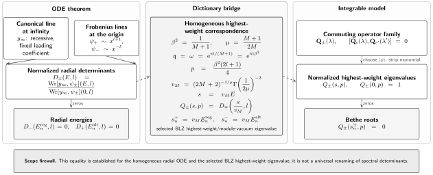
The determinant–Baxter bridge. ODE theory constructs normalized entire functions from one infinity line and each of two Frobenius origin lines. The middle passport fixes the sign reversal, parameter map, and spectral scale. Only after the homogeneous highest-weight correspondence is declared do the same entire functions become module-vacuum Baxter eigenvalues and their zeros become Bethe roots. No $TQ$ or transfer-matrix arrow is used on this page.

The large-variable asymptotic fixes the spectral scale

Writing $s$ as merely “proportional to $E$” leaves a physically relevant normalization unfixed. Put

$$a_0 = -\frac{ \Gamma(-\mu)\Gamma(\mu+\tfrac12) }{ \sqrt{\pi} }.$$

On the ODE side, as $|E|\to\infty$ with $|\arg(-E)|<\pi$,

$$\log D_-(E,l) \sim \frac{a_0}{2}(-E)^\mu.$$

The normalized module-vacuum Baxter eigenvalue has, as $|s|\to\infty$ in the corresponding cut sector,

$$\begin{aligned} \log Q_+(s,p) \sim{}& a_0(M+1) \\ &\times \Gamma\!\left(\frac{1}{2\mu}\right)^{2\mu} (-s)^\mu. \end{aligned}$$

Both powers use the principal logarithm on that sector: $(-z)^\mu=\exp[\mu\Log(-z)]$ with $-\pi<\arg(-z)<\pi$.

Set $E=s/v_M$ and match the two coefficients. This gives

$$v_M = (2M+2)^{-1/\mu} \Gamma\!\left(\frac{1}{2\mu}\right)^{-2}.$$

It is often convenient to retain the square-root scale

$$\nu_M = (2M+2)^{-1/(2\mu)} \Gamma\!\left(\frac{1}{2\mu}\right)^{-1}, \qquad v_M=\nu_M^2,$$

so that $\lambda=\nu_M\sqrt E$. The branch of $\sqrt E$ does not affect $Q_\pm$ because they are entire in $s=\lambda^2$.

Matching the leading asymptotic is necessary but not sufficient for the ODE/IM equality. The established correspondence also matches the functional relation, analyticity, zero distribution, and the normalization at zero. Page 5 exposes the functional part of that lock.

The sign reversal is controlled by one involution

The equation depends on $l$ only through $l(l+1)$ and is invariant under

$$l\longmapsto-1-l.$$

This exchanges the two Frobenius roles and gives

$$\begin{aligned} \Delta_+(E,l) &= \Delta_-(E,-1-l), \\ D_+(E,l) &= D_-(E,-1-l). \end{aligned}$$

Under the parameter map, the same involution is

$$p\longmapsto-p,$$

and the normalized module-vacuum eigenvalues obey, wherever both sides are finite,

$$Q_-(s,p)=Q_+(s,-p).$$

This explains, rather than merely memorizes, the correspondence $Q_\pm\leftrightarrow D_\mp$. The exceptional set is larger than the single repeated-exponent point: it is exactly

$$l+\frac12 = \pm\bigl[m_1+(M+1)m_2\bigr], \qquad m_1,m_2\in\mathbb Z_{\geq0}.$$

At these values the preferred Frobenius or normalization data can mix, develop poles, or require logarithmic solutions. The point $l=-1/2$ is the most visible member because the exponents coincide. Analytic continuation or a regularized basis is then required; the paired analysis belongs to Page 6.

Bethe roots inherit the radial spectrum

The determinant identity immediately converts zeros:

$$\begin{aligned} Q_+(s_n^+,p)=0 &\quad\Longleftrightarrow\quad \frac{s_n^+}{v_M} =E_n^{\mathrm{reg}}, \\ Q_-(s_n^-,p)=0 &\quad\Longleftrightarrow\quad \frac{s_n^-}{v_M} =E_n^{\mathrm{alt}}. \end{aligned}$$

For the regular real problem with nonexceptional $l>-1/2$, the first sequence is positive, discrete, and simple. Through the established dictionary this proves those properties for the roots of the selected vacuum $Q_+$-eigenvalue. It says nothing comparable about arbitrary states or arbitrary integrable models.

The Weyl law also transports directly:

$$E_n^{\mathrm{reg}} \asymp n^{1/\mu} \quad\Longrightarrow\quad s_n^+ \asymp n^{1/\mu}.$$

Thus the continuum Bethe roots have precisely the density required for an entire function of order $\mu$. The root divisor plus $Q_+(0,p)=1$ then reconstructs the function in the genus-zero range.

No Bethe equation has yet been used. On Page 5, evaluating the normalized $TQ$ identity at $s=s_n^\pm$ produces the phase constraint on neighboring rotated values. That condition is necessary, but roots alone still do not prove existence, admissibility, completeness, or the choice of integrable state.

Quartic highest-weight example

For $M=2$,

$$\beta^2=\frac13, \qquad \mu=\frac34, \qquad \mathfrak q=\ee^{\pi\ii/3},$$

and

$$v_2 = 6^{-4/3} \Gamma\!\left(\frac23\right)^{-2}.$$

At $l=0$, one has $p=1/12$, so

$$\begin{aligned} Q_+\!\left(s,\frac1{12}\right) &= D_{\mathrm D}\!\left(\frac{s}{v_2}\right), \\ Q_-\!\left(s,\frac1{12}\right) &= D_{\mathrm N}\!\left(\frac{s}{v_2}\right). \end{aligned}$$

The $Q_+$ roots are $v_2$ times the half-line Dirichlet levels, and the $Q_-$ roots are $v_2$ times the Neumann levels.

This example should not be confused with Page 3’s larger family $x^4+gx^2+\alpha x$. That family has an exact Symanzik parameter orbit, but no equality with the same BLZ $Q$-eigenvalues follows. A model, state, spectral scale, functional system, and matching asymptotic passport would all have to be supplied.

Common pitfalls

Calling every determinant a Q-function. Entirety and a spectral zero set are necessary ODE data, not an integrable-model identification. The operator, state, parameter map, scale, functional relation, asymptotics, and normalization must all match.

Confusing roots with spatial nodes. A Bethe root is a zero in $s$ of a scalar $Q$-eigenvalue. A node is a zero in $x$ of a wavefunction at fixed energy; a turning point is a zero of the classical momentum.

Forgetting the state. The elementary radial equation matches the highest-weight/module-vacuum eigenvalue. Higher qKdV states require ODEs with additional apparent singularities, often called monster potentials.

Treating the companion determinant as automatically self-adjoint. $D_+$ is a useful analytic connection function away from its exceptional parameters. Its zeros are a physical spectrum only after an admissible endpoint domain is declared; which of $D_\pm$ is Friedrichs changes at $l=-1/2$.

Exercises

1. Separate the three Q-objects. Explain why an operator $\mathbf Q(\lambda)$ is not determined by one eigenvalue, and why a scalar eigenvalue is not determined by its zeros without growth and normalization data.

Solution

An operator has eigenvalues on all states, together with their common eigenvectors and algebraic relations; one scalar function supplies only one diagonal entry. A zero divisor determines an entire function only up to a zero-free factor. In the present genus-zero range, the order bound reduces that factor to a constant, and $Q(0)=1$ fixes the constant.

2. Prove the radial zero criterion. For real nonexceptional $l>-1/2$, show both directions of

$$\Delta_-(E_*,l)=0 \quad\Longleftrightarrow\quad \begin{gathered} \text{one solution is regular at zero}\\ \text{and recessive at infinity} \end{gathered}.$$

Solution

The Wronskian vanishes exactly when $y(\,\cdot\,,E_*,l)$ and $\psi_+(\,\cdot\,,E_*,l)$ are linearly dependent. The first is recessive at infinity and the second spans the $x^{l+1}$ regular origin line in the stated range, so dependence produces one solution with both properties. Conversely, any solution with both properties must be proportional to each one-dimensional canonical line, so their Wronskian vanishes.

3. Recover the Page 1 pair. At $l=0$, derive the raw endpoint Wronskians and show that normalization gives $D_-=D_{\mathrm D}$ and $D_+=D_{\mathrm N}$.

Solution

With $\psi_+\sim x$ and $\psi_-\sim1$,

$$\begin{aligned} \Wr[y,\psi_+]\big|_{x=0} &=y(0,E), \\ \Wr[y,\psi_-]\big|_{x=0} &=-y'(0,E). \end{aligned}$$

Dividing each expression by its value at $E=0$ gives the normalized Dirichlet and Neumann endpoint functions. The two minus signs in the Neumann ratio cancel.

4. Check the zero-energy constants. Wherever both sides are finite, use Euler’s reflection formula to prove

$$\Delta_-(0,l)\Delta_+(0,l) = \frac{2l+1}{ \sin\!\left[\pi(2l+1)/(2M+2)\right] }.$$

Solution

Put $a=(2l+1)/(2M+2)$. Multiplication of the two displayed constants gives

$$\frac{2M+2}{\pi} \Gamma(1+a)\Gamma(1-a).$$

Since $\Gamma(1+a)\Gamma(1-a)=\pi a/\sin(\pi a)$, the product is $(2M+2)a/\sin(\pi a)$, which is the claimed expression. The identity then extends meromorphically in $l$.

5. Match the orders. Starting from $\beta^2=1/(M+1)$, show

$$\mu = \frac{M+1}{2M} = \frac{1}{2-2\beta^2}.$$

Why is $M>1$ exactly $0<\beta^2<1/2$?

Solution

Solving for $M$ gives $M=\beta^{-2}-1$. Therefore

$$\frac{M+1}{2M} = \frac{\beta^{-2}}{2(\beta^{-2}-1)} = \frac{1}{2-2\beta^2}.$$

For positive $M$, the inequality $M>1$ is equivalent to $\beta^{-2}>2$, hence $0<\beta^2<1/2$.

6. Derive the spectral scale. Match the two large-variable asymptotics and recover $v_M$.

Solution

Substituting $E=s/v_M$ into the ODE asymptotic gives the coefficient $a_0/(2v_M^\mu)$. Equating it to the Baxter coefficient yields

$$\frac{1}{2v_M^\mu} = (M+1) \Gamma\!\left(\frac{1}{2\mu}\right)^{2\mu}.$$

Solving for $v_M$ gives

$$v_M = (2M+2)^{-1/\mu} \Gamma\!\left(\frac{1}{2\mu}\right)^{-2}.$$

7. Translate the quartic passport. Compute $\beta^2,\mu,p,v_2$ for $M=2,l=0$ and identify both root sequences.

Solution

Direct substitution gives

$$\beta^2=\frac13, \qquad \mu=\frac34, \qquad p=\frac1{12},$$

and

$$v_2 = 6^{-4/3}\Gamma\!\left(\frac23\right)^{-2}.$$

The $Q_+$ roots are $v_2E_n^{\mathrm D}$ and the $Q_-$ roots are $v_2E_n^{\mathrm N}$.

8. Reject a premature identification. For $x^4+gx^2+\alpha x$, list data still missing before a radial determinant can be called one of the BLZ Baxter functions on this page.

Solution

One must supply an integrable model and commuting $Q$-operator, select a state, map $(g,\alpha)$ to model parameters, fix the spectral scale and zero normalization, match the entire-function asymptotics, and prove the same functional relation and analytic passport. Symanzik covariance alone provides none of those model-side data.

References

• R. J. Baxter, Exactly Solved Models in Statistical Mechanics, Academic Press, 1982, Chapters 9–10, for transfer matrices, $Q$-operators, and the finite-system origin of Bethe roots.
• V. V. Bazhanov, S. L. Lukyanov, and A. B. Zamolodchikov, “Integrable Structure of Conformal Field Theory II: Q-Operator and DDV Equation”, Communications in Mathematical Physics 190 (1997), 247–278, for the construction of the conformal $Q$-operators and their analytic eigenvalues.
• V. Bazhanov, S. Lukyanov, and A. Zamolodchikov, “Spectral Determinants for Schrödinger Equation and Q-Operators of Conformal Field Theory”, Journal of Statistical Physics 102 (2001), 567–576, for the primary generic-$p$ radial determinant correspondence.
• P. Dorey and R. Tateo, “On the Relation between Stokes Multipliers and the T–Q Systems of Conformal Field Theory”, Nuclear Physics B 563 (1999), 573–602, with erratum, for the Frobenius-Wronskian convention, normalization constants, exact spectral scale, and normalization-complete dictionary used here.
• V. V. Bazhanov, S. L. Lukyanov, and A. B. Zamolodchikov, “Higher-Level Eigenvalues of Q-Operators and Schrödinger Equation”, Advances in Theoretical and Mathematical Physics 7 (2003), 711–725, for the additional apparent singularities needed for higher-state $Q$-eigenvalues.
• P. Dorey, C. Dunning, and R. Tateo, “The ODE/IM Correspondence”, Journal of Physics A 40 (2007), R205–R283, especially Sections 5.1–5.4 for the determinant, parameter, state, and analyticity dictionaries.
• E. Delabaere and J.-M. Rasoamanana, “Resurgent Deformations for an Ordinary Differential Equation of Order 2”, Pacific Journal of Mathematics 223 (2006), 35–93, for global Stokes–Sibuya analysis of polynomial-over-$x^2$ equations with nontrivial origin monodromy.