Seiberg–Witten Curves, Differentials, Cycles, and Special Geometry

Page 1 left the infrared theory in an abstract form: a local system of charges, its integral skew pairing, and an additive central charge $Z_u$. Seiberg–Witten geometry realizes that package by integration. Charges become oriented cycles, the skew pairing becomes topological intersection, and the central charge becomes a period of a distinguished meromorphic one-form.

The word distinguished does most of the work. An algebraic curve alone does not fix the periods, their units, the integral charge lattice, or even which part of the curve’s homology is physical. The differential, polarization, residues, asymptotics, and parameter map must accompany it. This page constructs that normalization-complete datum and tests it on pure $SU(2)$ theory. Everything remains classical and undeformed: the Omega background starts only on Page 3.

Page question

How does a family of curves with a specified differential and integral cycle lattice turn the abstract central charge of Page 1 into local special coordinates with controlled monodromy?

Status ledger

Statement used on this page	Status
A Seiberg–Witten solution needs a curve, differential, and physical integral cycle data	Structural statement
The dynamical particle lattice equals all of $H_1(\Sigma_u,\mathbb Z)$	Model-dependent; it already fails in the unit-probe normalization of pure $SU(2)$ below
Flavor masses are residue periods	Exact after the residue-to-mass convention is declared
$\partial_{u^k}\lambda_{\mathrm{SW}}$ is holomorphic modulo an exact form	Defining cohomological property at fixed ultraviolet parameters
$a_{D,i}=\partial\mathcal F/\partial a^i$	Local statement in a nonsingular electric frame
$\operatorname{Im}\tau>0$	Physical positivity condition, obtained from the polarized period matrix
A vanishing cycle labels a massless particle	Conditional on that charge being populated by a BPS state
Pure-$SU(2)$ periods satisfy a second-order Picard–Fuchs ODE	Exact classical statement in the convention declared below
A Picard–Fuchs ODE is a quantum spectral equation	False; its independent variable is a Coulomb modulus
WKB cycles equal gauge charges	Still deferred to Page 6

A curve equation is only the first line of the answer

Let $\mathcal B^\circ=\mathcal B\setminus\Delta$ be the Coulomb branch with its discriminant locus removed. A useful schematic form of the classical Seiberg–Witten datum is

$$\begin{gathered} \pi:\mathcal S\longrightarrow\mathcal B^\circ, \qquad \pi^{-1}(u)=\Sigma_u, \qquad D_u=\sum_p m_p p, \\ \lambda_{\mathrm{SW}}(u) \in H^0\!\left( \Sigma_u, K_{\Sigma_u}(D_u) \right), \qquad \widehat\Gamma_u \dashrightarrow H_1\!\left( \Sigma_u\setminus |D_u|, \mathbb Z \right). \end{gathered}$$

Here $\Sigma_u$ is a smooth compact Riemann surface and $D_u$ is an effective pole divisor: $m_p$ records the allowed pole order and $|D_u|$ denotes its reduced support. Thus the notation includes the second-kind double poles in the pure example below. The dashed arrow means “specified realization,” not “automatic equality.” Depending on the construction, the physical lattice can be a sublattice, a quotient, a subquotient, or an anti-invariant/Prym part defined by an actual covering involution. Other realizations use a relative homology group with endpoints at marked points; the homology functor is part of the model, not a universal default.

The remaining entries of the passport are just as important:

Datum	What it fixes
Family $\pi:\mathcal S\to\mathcal B^\circ$	How the complex structure varies with the Coulomb vacuum
Pole divisor $D$ and $\lambda_{\mathrm{SW}}$	Central-charge units, mass residues, and special coordinates
Particle lattice, period lattice, and polarization	Which cycle classes represent dynamical charges, whether periods extend to a larger probe lattice, and how they pair
Ultraviolet parameter map	Which coefficients are moduli, masses, couplings, or the scale $\Lambda$
Weak-coupling asymptotics	The physical normalization and identification of the electric frame
Paths and loop orientations	The actual monodromy matrices rather than their conjugacy classes

The charge lattice first carries an integral alternating Dirac pairing. In an Abelian-fibration realization, a polarization is the corresponding positive integral $(1,1)$ Riemann form; its elementary divisors define the polarization type. A principal polarization has all elementary divisors equal to one, so a basis with unit pairings $A_i\circ B^j=\delta_i{}^j$ exists.

The genus $g(\Sigma_u)$ therefore need not equal the gauge rank $r$. It does in elementary hyperelliptic examples where the relevant compact periods fill a Jacobian. In a higher cover one can have $r<g$, with only a polarized Abelian subvariety carrying the physical periods. A puncture supplies a flavor direction only when theory data select its loop class and declare its residue to be a mass; punctures do not do so automatically.

Same equation, different theory data

A birational change of variables is harmless only after the differential and cycles are transported with it. An isogeny can change the integral polarization. Closely related global forms such as $SU(2)$ and $SO(3)$ can require different integral lattices and related, isogenous elliptic curves. Equality of a bare equation, when it occurs, is not a complete equivalence claim.

Cycles are local, integral, and oriented

Work first on a simply connected patch $U\subset\mathcal B^\circ$. Assume for the moment that the rank-$2r$ period lattice $\Gamma_{\mathrm{per}}$ has a principal polarization. Choose locally constant cycles

$$A_i, B^i, \qquad i=1,\ldots,r,$$

with intersection convention

$$\begin{aligned} A_i\circ A_j&=0, & B^i\circ B^j&=0, & A_i\circ B^j&=\delta_i{}^j. \end{aligned}$$

Then a gauge period-lattice class is represented by

$$\gamma_{\mathrm{per}} = n_e^iA_i+n_{m,i}B^i,$$

and geometric intersection reproduces the convention of Page 1:

$$\gamma_{\mathrm{per}}\circ\gamma'_{\mathrm{per}} = \boldsymbol n_e\mathbin{\cdot}\boldsymbol n_m' - \boldsymbol n_m\mathbin{\cdot}\boldsymbol n_e'.$$

If $\Gamma_{\mathrm{per}}$ has a nonprincipal polarization, the right side contains positive integer elementary divisors $d_i$. Even when $\Gamma_{\mathrm{per}}$ is principal, its embedded dynamical sublattice $\Gamma_{\mathrm{em}}$ can have nontrivial elementary divisors, as in the pure-$SU(2)$ example below. These integers are integral theory data; they cannot be removed by a complex change of basis.

If $\lambda_{\mathrm{SW}}$ has simple poles, theory data may select independent small positively oriented loops $C_a$ around marked points. Their mutual intersections vanish, and they can be arranged to pair trivially with the compact gauge cycles. Those selected loops whose residues have the prescribed mass normalization realize flavor directions in the radical of the full skew pairing. Relations among puncture loops—most simply $\sum_a C_a=0$ on a punctured compact curve—mean that one should not count every small loop as an independent flavor charge.

After choosing the same kind of local flavor splitting as on Page 1, the selected compact and puncture cycles form an extended period lattice

$$\widehat\Gamma_{\mathrm{per}} = \Gamma_{\mathrm{per}} \oplus \Gamma_{\mathrm f}.$$

The physical $\widehat\Gamma$ is realized in this target by the model-specific sublattice, quotient, or subquotient map declared in the geometric passport; an injection is not assumed universally.

As $u$ moves, the cycles are transported horizontally by the Gauss–Manin connection. Returning around a noncontractible loop can return a different integral basis. Thus $A_i$ and $B^i$ are local sections of a homology local system, not globally fixed contours drawn once and for all.

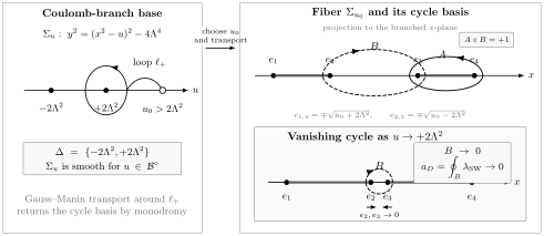
The family and its cycles in the pure-$SU(2)$ convention used below. The base has discriminant points $u=\pm2\Lambda^2$. The stem from $u_0$ to the local counterclockwise loop is a chosen connector, traversed out and back. Over $u_0$, the quartic model has four branch points and a local basis with $A\circ B=+1$. The dashed $B$ contour changes sheet at each cut; its chosen lift meets the solid $A$ lift once on $\Sigma_{u_0}$. Gauss–Manin transport around $u=+2\Lambda^2$ changes the basis, while $B$ itself collapses as the monopole point is approached.

The differential carries the physical normalization

At fixed masses and couplings, the defining variation property is best stated in punctured meromorphic de Rham cohomology. Let $\nabla$ denote the Gauss–Manin connection on that fiberwise cohomology local system. The differential defines a class and its Coulomb-modulus variation is holomorphic:

$$\begin{gathered} [\lambda_{\mathrm{SW}}] \in H^1_{\mathrm{dR}}\!\left( \Sigma_u\setminus|D_u| \right), \\ \nabla_{\partial/\partial u^k} [\lambda_{\mathrm{SW}}] = [\omega_k], \qquad \omega_k\in H^{1,0}(\Sigma_u). \end{gathered}$$

After choosing a local trivialization of the family, this says

$$\left. \frac{\partial\lambda_{\mathrm{SW}}}{\partial u^k} \right|_{m,\tau_{\mathrm{UV}}\ \mathrm{or}\ \Lambda} = \omega_k+\dd_x f_k,$$

where $f_k$ is single-valued and meromorphic. The exact term matters in an algebraic representative but integrates to zero on every closed cycle. Taking the derivative of a period along a horizontal cycle gives

$$\begin{aligned} \frac{\partial}{\partial u^k} \oint_{A_i}\lambda_{\mathrm{SW}} &= \oint_{A_i}\omega_k, \\ \frac{\partial}{\partial u^k} \oint_{B^i}\lambda_{\mathrm{SW}} &= \oint_{B^i}\omega_k. \end{aligned}$$

Several superficially similar modifications are not equivalent:

Change of differential	Effect
$\lambda_{\mathrm{SW}}\mapsto\lambda_{\mathrm{SW}}+\dd_x f$ with single-valued $f$	No change to closed periods
Multiplication by a constant	Rescales all central charges and BPS masses
Addition of a holomorphic one-form	Generally shifts electric and magnetic periods
Addition of a mass-dependent exact form	Preserves closed periods but can simplify residue representatives
Multivalued “primitive” $f$	Not an innocuous exact shift; its continuation can carry periods

For matter theories, the residue convention supplies the flavor part of the central charge. With positively oriented $C_a$,

$$\oint_{C_a}\lambda_{\mathrm{SW}} = 2\pi\ii\, \operatorname{Res}_{p_a} \lambda_{\mathrm{SW}} = \kappa_a{}^f m_f.$$

The fixed matrix $\kappa_a{}^f$ depends on flavor-weight and mass conventions. It is often a signed half-integer or integer matrix rather than the identity. Declaring only the locations of poles, without their residues, leaves the mass normalization unfinished.

Periods realize the Page 1 central charge

We absorb every overall factor into $\lambda_{\mathrm{SW}}$ and define

$$a^i(u) = \oint_{A_i}\lambda_{\mathrm{SW}}, \qquad a_{D,i}(u) = \oint_{B^i}\lambda_{\mathrm{SW}}.$$

For a class in the declared extended period lattice,

$$\gamma = n_e^iA_i+n_{m,i}B^i+s^aC_a,$$

linearity of integration gives

$$\begin{aligned} Z_\gamma(u) &= \oint_\gamma\lambda_{\mathrm{SW}} \\ &= n_e^i a^i(u) + n_{m,i}a_{D,i}(u) + s^a\kappa_a{}^f m_f. \end{aligned}$$

Restricting this equality to the embedded dynamical lattice is the geometric realization of the additive homomorphism on Page 1. It also exposes why an arbitrary rescaling of the differential is physical: it rescales $Z_\gamma$ and therefore every BPS mass.

Normalization placement

Many sources instead write $a=(2\pi\ii)^{-1}\oint_A\lambda$ with an unnormalized algebraic differential $\lambda$. We place that factor inside $\lambda_{\mathrm{SW}}$. Either convention is valid, but combining the period definition from one source with the differential from another changes every answer by $2\pi\ii$.

Riemann bilinear relations generate special geometry

For a transparent surface derivation, first suppose that $r=g$ and that $\{A_i,B^i\}_{i=1}^r$ is a complete symplectic basis of $H_1(\Sigma_u,\mathbb Z)$. If $r<g$, the same conclusion follows from the Riemann relations on the chosen polarized $r$-dimensional Abelian variety—often a Prym—not by truncating the bilinear sum on $\Sigma_u$. The corresponding selected subspace of holomorphic forms plays the role of the forms below.

Suppose the $r\times r$ matrix

$$\mathsf A^i{}_k = \frac{\partial a^i}{\partial u^k} = \oint_{A_i}\omega_k$$

is invertible. This is the local nondegeneracy condition that permits $a^i$ to serve as coordinates. Define the holomorphic differentials

$$\eta_j = \frac{\partial\lambda_{\mathrm{SW}}}{\partial a^j} \quad\text{in cohomology}.$$

They are normalized by

$$\oint_{A_i}\eta_j = \delta_i{}^j.$$

Their $B$ periods form the effective coupling matrix:

$$\tau_{ij} = \oint_{B^i}\eta_j = \frac{\partial a_{D,i}}{\partial a^j}.$$

Because the displayed cycles form a complete basis, the first Riemann bilinear relation makes this matrix symmetric, and the positivity relation makes its imaginary part positive definite:

$$\tau_{ij}=\tau_{ji}, \qquad \operatorname{Im}\tau>0.$$

Symmetry implies that the holomorphic one-form $a_{D,i}\,\dd a^i$ on the coordinate patch is closed. The holomorphic Poincaré lemma therefore supplies a local prepotential $\mathcal F$:

$$a_{D,i} = \frac{\partial\mathcal F}{\partial a^i}, \qquad \tau_{ij} = \frac{\partial^2\mathcal F} {\partial a^i\partial a^j}.$$

The corresponding rigid special Kähler potential and metric can be written locally as

$$\begin{aligned} K &= \operatorname{Im} \left( \overline{a^i}a_{D,i} \right), \\ \dd s^2 &= \operatorname{Im}\tau_{ij}\, \dd a^i\, \dd\overline{a^j}, \end{aligned}$$

up to the overall positive factor chosen in the four-dimensional action. This is why positivity of the period matrix is a physical condition rather than a decorative property of the auxiliary curve.

The prepotential is not generally a single global function on $\mathcal B^\circ$. It belongs to a local electric frame. After a duality transformation it changes by the appropriate Legendre and quadratic generating terms, while the special Kähler geometry remains well defined.

Monodromy changes components, not the central charge

Order gauge periods and period-lattice charge components as in the extended frame of Page 1:

$$\Pi = \begin{pmatrix} \boldsymbol a_D\\ \boldsymbol a \end{pmatrix}, \qquad q = \left( \boldsymbol n_m, \boldsymbol n_e \right), \qquad Z=q\Pi.$$

In the principal frame used here, let

$$M = \begin{pmatrix} P&Q\\ R&S \end{pmatrix} \in Sp(2r,\mathbb Z),$$

active transport of the period section and the contragredient relabeling of charge components are

$$\Pi'=M\Pi, \qquad q'=qM^{-1}.$$

Consequently $q'\Pi'=q\Pi$, while

$$\tau' = (P\tau+Q) (R\tau+S)^{-1}.$$

The displayed $M$ acts on a principal $\Gamma_{\mathrm{per}}$. If the period polarization itself has type $D=\operatorname{diag}(d_i)$, monodromy instead preserves its integral alternating matrix $J_D$ and need not be represented by the unit-form $Sp(2r,\mathbb Z)$ matrices above. A second possibility is a principal $\Gamma_{\mathrm{per}}$ with a nonprincipal embedded $\Gamma_{\mathrm{em}}$: the ambient symplectic monodromy stabilizes that sublattice, while a dynamical-lattice-adapted basis represents it by matrices preserving the corresponding $J_{D_{\mathrm{dyn}}}$. With flavor punctures, the compact gauge block remains pairing-preserving, but $a$ and $a_D$ can also acquire integral linear combinations of mass periods. The full continuation is then an affine extension of the displayed gauge action.

Around a simple nodal degeneration, let the primitive vanishing cycle be

$$\delta=n_eA+n_mB$$

at rank one. We define the positive loop and active cycle convention by

$$T_\delta(\gamma) = \gamma- (\gamma\circ\delta)\delta.$$

Then the ordered period vector transforms by

$$M_\delta = \begin{pmatrix} 1+n_en_m&n_e^2\\ -n_m^2&1-n_en_m \end{pmatrix}.$$

This formula is convention-sensitive. Reversing the intersection form, reversing the base loop, or switching between active period transport and passive charge relabeling inverts or conjugates the displayed matrix. A paper that lists only a matrix without these declarations has not supplied a reproducible monodromy convention.

Pure SU(2) in the Page 1 normalization

We now fix every entry for pure $SU(2)$ theory. The scale $\Lambda$ is the curve-normalized representative of the complexified dynamical scale; its multiplicative relation to a particular renormalization scheme is conventional. The quartic depends only on $\Lambda^4$; writing $\Lambda^2$ chooses a square root, and reversing that choice exchanges the labels of the two finite singularities. Our passport is

Item	Convention
Coulomb coordinate	$u\sim a_{\mathrm{cl}}^2$ at weak coupling
Electric unit	A fundamental probe has charge one; the $W$ multiplet has charge two
Central-charge normalization	$M_\gamma=
Cycle orientation	$A\circ B=+1$
Period order	$\Pi=(a_D,a)^T$
Weak electric period	$a(u)\sim\sqrt u$ on the positive real sheet
Scale root	$\Lambda^4$ is invariant; choose $\Lambda^2>0$ on the displayed real slice
Strong-coupling points	$u_\pm=\pm2\Lambda^2$
Monodromy action	Counterclockwise active continuation of periods from a large positive base point

A convenient form of the curve and its normalized differential is

$$\Sigma_u: \qquad \Lambda^2 \left( z+\frac1z \right) = x^2-u, \qquad \lambda_{\mathrm{SW}} = \frac{1}{2\pi\ii} x\frac{\dd z}{z}.$$

The dimensions are

$$[x]=[\Lambda]=[\lambda_{\mathrm{SW}}]=1, \qquad [u]=2,$$

so every period has the required mass dimension. Introducing

$$y = \Lambda^2 \left( z-\frac1z \right)$$

gives the equivalent quartic presentation

$$y^2 = (x^2-u)^2-4\Lambda^4, \qquad \lambda_{\mathrm{SW}} = \frac{x^2\,\dd x}{\pi\ii\,y}.$$

The second expression follows from $2x\,\dd x=y\,\dd z/z$. It is the form projected in the figure. The compact quartic has two unbranched points above $x=\infty$. At each one, $\lambda_{\mathrm{SW}}$ has a second-kind double pole with zero residue. The principally polarized homology

$$\Gamma_{\mathrm{per}} = H_1(\Sigma_u,\mathbb Z) = \mathbb ZA\oplus\mathbb ZB, \qquad A\circ B=1,$$

is the enlarged period lattice that includes a unit electric probe. Page 1’s dynamical particle lattice is instead

$$\widehat\Gamma = 2\mathbb ZA\oplus\mathbb ZB \hookrightarrow \Gamma_{\mathrm{per}}.$$

Its elementary divisor is two because $(2A)\circ B=2$: the $W$ multiplet has charge $2A$, whereas the monopole has charge $B$. Thus full homology and the Page 1 particle lattice are not being identified. There are no flavor-residue directions in this pure theory.

The variation is holomorphic in cohomology

At fixed $z$, differentiating $x^2=u+\Lambda^2(z+z^{-1})$ is immediate:

$$\left. \frac{\partial\lambda_{\mathrm{SW}}}{\partial u} \right|_z = \frac{1}{4\pi\ii x} \frac{\dd z}{z} = \frac{\dd x}{2\pi\ii\,y}.$$

The final form is the unique holomorphic differential on this elliptic curve, up to scale. If one differentiates the quartic representative at fixed $x$ instead, the answer looks different but has the same cohomology class:

$$\left. \frac{\partial\lambda_{\mathrm{SW}}}{\partial u} \right|_x = \frac{\dd x}{2\pi\ii\,y} - \dd_x \left( \frac{x}{2\pi\ii\,y} \right).$$

This identity is a concrete reason to formulate the defining variation property modulo exact forms. The derivative depends on how the family was locally trivialized; the period derivative does not.

Four branch points give genus one and two finite degenerations

Choose the phase of the curve-normalized scale so that $\Lambda^2>0$. For $u_0>2\Lambda^2$ on this real slice, the quartic branch points on the real $x$ axis are

$$\begin{aligned} e_1&=-\sqrt{u_0+2\Lambda^2}, & e_2&=-\sqrt{u_0-2\Lambda^2}, \\ e_3&=+\sqrt{u_0-2\Lambda^2}, & e_4&=+\sqrt{u_0+2\Lambda^2}. \end{aligned}$$

The compactified curve is a double cover of the $x$ sphere branched at four simple points. Riemann–Hurwitz gives

$$2g(\Sigma)-2 = 2(-2)+4,$$

hence $g=1$. The reduced discriminant is

$$\Delta_{\mathrm{red}}(u) = u^2-4\Lambda^4.$$

At $u=+2\Lambda^2$, the inner branch points $e_2$ and $e_3$ collide at zero. At $u=-2\Lambda^2$, the other pairing degenerates after analytic continuation. These are the two finite singular fibers. The point $u=\infty$ is the weak-coupling singular point of the compactified $u$-sphere.

Choose $A$ and $B$ as in the figure, with the orientation adjusted so that $A\circ B=+1$. The $B$ cycle collapses at $u_+$, and therefore

$$a_D(u) = \oint_B\lambda_{\mathrm{SW}} \longrightarrow0 \qquad \text{as} \qquad u\longrightarrow+2\Lambda^2.$$

Geometry has identified a vanishing charge. The statement that a monopole hypermultiplet of that charge is actually present is additional physical information, albeit information realized in this theory.

The weak period is an exact hypergeometric function

At large positive $u$, take the $A$ cycle to project to $|z|=1$ and write $z=e^{\ii\theta}$. On the sheet with $x\sim+\sqrt u$,

$$x(\theta) = \sqrt{ u+2\Lambda^2\cos\theta }.$$

The period becomes an elementary angular average:

$$a(u) = \frac1{2\pi} \int_0^{2\pi} \sqrt{ u+2\Lambda^2\cos\theta } \,\dd\theta.$$

Expanding uniformly for $|u|>2|\Lambda|^2$ gives

$$\begin{aligned} a(u) &= \sqrt u\, {}_2F_1\!\left( -\frac14, \frac14; 1; \frac{4\Lambda^4}{u^2} \right) \\ &= \sqrt u \left[ 1 - \frac{\Lambda^4}{4u^2} - \frac{15\Lambda^8}{64u^4} + O\!\left( \frac{\Lambda^{12}}{u^6} \right) \right]. \end{aligned}$$

This checks the Page 1 convention $u\sim a^2$ rather than the older normalization $a\sim\sqrt{2u}$. It also gives an exact analytic germ, not merely an instanton-like formal series.

The second period has a logarithm at weak coupling. With the same path and branch conventions,

$$a_D(u) = \frac{4\ii}{\pi} a(u) \log\!\frac{a(u)}{\Lambda} + c_{\mathrm{lin}}a(u) + O\!\left( \frac{\Lambda^4}{a(u)^3} \right).$$

Its linear coefficient is fixed once the $B$ cycle, logarithm branch, and curve-scale convention are fixed. An allowed integral-frame change $B\mapsto B+kA$, or a rescaling convention for $\Lambda$, shifts that coefficient without changing the monodromy at infinity.

Picard–Fuchs turns the period problem into an ODE

The hypergeometric equation for the preceding $A$ period is equivalent to

$$\left[ \frac{\dd^2}{\dd u^2} + \frac{1}{4(u^2-4\Lambda^4)} \right] \Pi(u) = 0, \qquad \Pi\in\{a_D,a\}.$$

Both periods obey the same equation because Picard–Fuchs reduction acts on the two-dimensional cohomology local system before a cycle is chosen. The equation has regular singularities at $u=\pm2\Lambda^2$ and $u=\infty$. Near a finite discriminant point, one solution vanishes linearly and its companion has a constant plus a term proportional to $(u-u_\pm)\log(u-u_\pm)$. At infinity the two behaviors are $\sqrt u$ and $\sqrt u\log u$.

This is a classical period ODE. Its independent variable is the vacuum coordinate $u$; there is no wavefunction, boundary condition, spectral energy, or deformation parameter $\hbar$. The ODE determines a complex two-dimensional solution space, but the curve, differential, integral cycles, and weak asymptotics are still needed to identify the physical pair $(a_D,a)$ inside that space.

Three independent checks

The same normalization is tested in three ways: the $A$ period has $a\sim\sqrt u$, the differential variation is holomorphic modulo exact forms, and the logarithmic companion produces the expected integral monodromy. Agreement of only one check is not enough to certify a borrowed formula.

Vanishing cycles reproduce the three monodromies

Keep the large positive base point, counterclockwise loops, and the ordered vector $\Pi=(a_D,a)^T$. Choose the paths so that the vanishing charges are

$$\delta_+ = B, \qquad \delta_- = -2A+B.$$

Thus $Z_{\delta_+}=a_D$ and $Z_{\delta_-}=a_D-2a$. The Picard–Lefschetz formula gives

$$M_+ = \begin{pmatrix} 1&0\\ -1&1 \end{pmatrix}, \qquad M_- = \begin{pmatrix} -1&4\\ -1&3 \end{pmatrix}.$$

With the stated path ordering,

$$M_\infty = M_+M_- = \begin{pmatrix} -1&4\\ 0&-1 \end{pmatrix}.$$

The last matrix also follows directly from the weak-coupling logarithm:

$$a\longmapsto-a, \qquad a_D\longmapsto-a_D+4a.$$

Every matrix has determinant one and preserves the intersection form. The upper-right entry is four, not two, on the present unit-probe period lattice; the Page 1 dynamical lattice is its index-two sublattice and assigns charge two to the $W$ multiplet. By contrast, the original 1994 paper prints the lattice-adapted matrices below. The integral part of the conversion is

$$D = \begin{pmatrix} 1&0\\ 0&2 \end{pmatrix}, \qquad \Pi_{\mathrm{dyn}}=D\Pi, \qquad M_{\mathrm{dyn}}=DMD^{-1}.$$

Consequently that paper prints

$$M_+^{\mathrm{SW}} = \begin{pmatrix} 1&0\\ -2&1 \end{pmatrix}, \qquad M_\infty^{\mathrm{SW}} = \begin{pmatrix} -1&2\\ 0&-1 \end{pmatrix}.$$

That passport changes both period normalization and the integral charge/cycle lattice—an isogeny-type change. A common scalar rescaling of $(a_D,a)$ alone cannot change a monodromy matrix. Copying an older matrix while retaining the present $a\sim\sqrt u$ period lattice would therefore mix two passports.

Changing the path to the dyon point can replace $\delta_-=(-2,1)$ by a duality-equivalent representative such as $(2,1)$ and conjugate the matrix. The invariant content is the integral local system with its chosen base point and path system, not an isolated charge vector printed without that context.

What the geometry determines—and what it does not

The classical construction has now delivered

$$\begin{aligned} (\widehat\Gamma_u,\circ,Z_u) &\dashrightarrow (\widehat\Gamma_{\mathrm{per},u},\circ,Z_u), \\ (\widehat\Gamma_{\mathrm{per},u},\circ,Z_u) &\longleftarrow (\Sigma_u,\lambda_{\mathrm{SW}},\{A_i,B^i,C_a\}). \end{aligned}$$

Together with local special coordinates, the effective coupling, and monodromy. The dashed arrow allows the sublattice, quotient, and subquotient realizations declared at the start of the page. The extended period lattice may coincide with the particle–flavor lattice or may be an enlargement, as it is in the pure-$SU(2)$ normalization just used. The geometry does not by itself determine all of the following:

Missing conclusion	Additional input required
Which lattice charges are occupied by stable BPS particles	Chamber-dependent BPS spectrum
Which Wilson–’t Hooft lines are genuine	Global form and line-operator data
An Omega-deformed partition function	Page 3
A twisted superpotential	NS limit on Page 4
A quantum operator and ordering	Page 5
Equality with WKB cycles and periods	Explicit dictionary on Page 6
An accessory-parameter relation	Page 7
A complete exact spectrum	Boundary and nonperturbative completion on Page 8

In particular, a zero of a period is a geometric necessary condition for a state of that charge to become massless. It is not a proof that the charge is populated. Likewise, the Picard–Fuchs equation knows the complex variation of periods but not the four-dimensional spectrum.

A normalization ledger for any new curve

Before using a Seiberg–Witten curve from the literature, fill every row:

Question	Required declaration
Which theory?	Gauge algebra and global form, matter, masses, coupling or scale
Which vacuum coordinates?	The map from curve coefficients to $u_k$
Which curve family?	Equation, compactification, punctures, discriminant
Which differential?	Full formula, overall factor, poles, residues, exact-form convention
Which particle and period cycles?	Dynamical sublattice or subquotient, any enlarged probe lattice, and both polarizations
Which basis?	Cycle orientations, intersection signs, and order of periods
Which weak frame?	Asymptotics that identify electric variables
Which loops?	Base point, branch cuts, path ordering, and active/passive monodromy convention
Which status?	Classical, deformed, all-orders, resummed, or conjecturally complete

Only after these rows agree may two period formulas be compared term by term.

Common pitfalls

Calling an algebraic equation “the Seiberg–Witten solution.” The equation supplies a family of Riemann surfaces. Without the differential, physical integral lattice, residue map, and asymptotic normalization, it does not yet supply central charges.

Equating genus with gauge rank by definition. Equality holds in many hyperelliptic examples, including the pure-$SU(2)$ curve above. In general the physical Abelian variety can be a Prym or another polarized subvariety, and $r$ can be smaller than the genus of an auxiliary spectral cover.

Treating every change of differential as exact. A single-valued total derivative has zero closed periods. A rescaling or addition of a holomorphic form changes central charges and must be fixed by physical normalization.

Confusing $\tau_{\mathrm{UV}}$ with $\tau_{ij}(u)$. The first is microscopic theory data in a conformal theory. The second is the vacuum-dependent period matrix $\partial a_{D,i}/\partial a^j$ of the infrared Abelian theory.

Reading the Picard–Fuchs equation as a Schrödinger equation. It is an ODE for classical periods as functions of moduli. A quantum curve requires an independent deformation, polarization, operator ordering, and boundary problem.

Mixing the two standard pure-SU(2) passports. The older convention has $a\sim\sqrt{2u}$ and different printed monodromy entries. Rescale the differential, charge basis, scale, and matrices together; never change just one line.

Exercises

1. Recover the genus from the covering map

Use Riemann–Hurwitz to determine the genus of

$$y^2=(x^2-u)^2-4\Lambda^4$$

for $u^2\neq4\Lambda^4$. What changes at a finite discriminant point?

Solution

The projection $(x,y)\mapsto x$ has degree two. For a smooth quartic with four distinct roots, each root is a simple ramification point with ramification index two. Riemann–Hurwitz gives

$$2g-2 = 2(2\cdot0-2) + 4(2-1) = 0,$$

so $g=1$. At $u=+2\Lambda^2$, the roots $\pm\sqrt{u-2\Lambda^2}$ collide; at $u=-2\Lambda^2$, the analytically continued complementary pair collides. The smooth torus degenerates to a nodal curve and one one-cycle vanishes.

2. Compare two derivatives of the differential

Starting from

$$\Lambda^2(z+z^{-1})=x^2-u, \qquad \lambda_{\mathrm{SW}} = \frac{x}{2\pi\ii}\frac{\dd z}{z},$$

compute $\partial_u\lambda_{\mathrm{SW}}$ first at fixed $z$ and then at fixed $x$. Verify the exact-form relation printed in the text.

Solution

At fixed $z$, $2x\,\partial_u x=1$, so

$$\left. \partial_u\lambda_{\mathrm{SW}} \right|_z = \frac{1}{4\pi\ii x} \frac{\dd z}{z}.$$

Differentiating the curve at fixed $u$ gives $2x\,\dd x=y\,\dd z/z$, hence

$$\left. \partial_u\lambda_{\mathrm{SW}} \right|_z = \frac{\dd x}{2\pi\ii y}.$$

In the quartic form, $\lambda_{\mathrm{SW}}=x^2\dd x/(\pi\ii y)$ and $y^2=(x^2-u)^2-4\Lambda^4$. At fixed $x$,

$$\partial_u\!\left(\frac1y\right) = \frac{x^2-u}{y^3},$$

so

$$\left. \partial_u\lambda_{\mathrm{SW}} \right|_x = \frac{x^2(x^2-u)}{\pi\ii y^3}\,\dd x.$$

On the other hand,

$$\dd_x\!\left(\frac{x}{y}\right) = \left[ \frac1y - \frac{2x^2(x^2-u)}{y^3} \right]\dd x.$$

Rearranging proves

$$\left. \partial_u\lambda_{\mathrm{SW}} \right|_x = \frac{\dd x}{2\pi\ii y} - \dd_x\!\left(\frac{x}{2\pi\ii y}\right).$$

3. Separate exact shifts from mass shifts

Let $f$ be a single-valued meromorphic function on $\Sigma_u$. Show that replacing $\lambda_{\mathrm{SW}}$ by $\lambda_{\mathrm{SW}}+\dd f$ changes neither a closed period nor a residue. Why does the same conclusion fail for addition of a nonzero holomorphic one-form?

Solution

For every closed cycle $\gamma$ avoiding the poles,

$$\oint_\gamma\dd f=0$$

because $f$ returns to the same value. Locally, the derivative of a Laurent series has no coefficient of $(z-z_0)^{-1}\dd z$, so $\operatorname{Res}_{z_0}\dd f=0$. Thus both gauge periods and flavor residues are unchanged.

A nonzero holomorphic one-form is closed but generally not exact. Its $A$ and $B$ periods need not vanish, so adding it changes $a$, $a_D$, the central charges, and potentially the weak-coupling normalization.

4. Put flavor loops in the radical

Let $C_a$ and $C_b$ be disjoint small loops around two punctures. Show that they pair trivially with each other and with compact cycles chosen away from the punctures. Relate their periods to masses and state one global homology relation.

Solution

The loops can be represented in disjoint small disks, so $C_a\circ C_b=0$. A compact gauge cycle can be deformed away from those disks, giving $A_i\circ C_a=B^i\circ C_a=0$. Hence the span of the puncture loops lies in the radical of the intersection pairing.

For positive orientation,

$$\oint_{C_a}\lambda_{\mathrm{SW}} = 2\pi\ii\, \operatorname{Res}_{p_a} \lambda_{\mathrm{SW}},$$

which is a declared linear combination of flavor masses. On a compact surface with all punctures removed, the boundary of the complement of small disks yields the relation $\sum_a C_a=0$. Thus only an independent subset represents flavor directions.

5. Derive the first two weak-coupling corrections

Expand the angular integral for $a(u)$ through order $\Lambda^8/u^4$.

Solution

Set $\varepsilon=2\Lambda^2/u$. Then

$$a(u) = \sqrt u\, \left\langle (1+\varepsilon\cos\theta)^{1/2} \right\rangle,$$

where $\langle\cdot\rangle$ is the average over $0\leq\theta<2\pi$. Odd powers average to zero, while

$$\left\langle\cos^2\theta\right\rangle = \frac12, \qquad \left\langle\cos^4\theta\right\rangle = \frac38.$$

Using $\binom{1/2}{2}=-1/8$ and $\binom{1/2}{4}=-5/128$ gives

$$\begin{aligned} a(u) &= \sqrt u \left[ 1 - \frac{\varepsilon^2}{16} - \frac{15\varepsilon^4}{1024} + O(\varepsilon^6) \right] \\ &= \sqrt u \left[ 1 - \frac{\Lambda^4}{4u^2} - \frac{15\Lambda^8}{64u^4} + O\!\left( \frac{\Lambda^{12}}{u^6} \right) \right]. \end{aligned}$$

6. Verify the Picard–Fuchs equation

Let

$$F(\zeta) = {}_2F_1\!\left( -\frac14, \frac14; 1; \zeta \right), \qquad \zeta=\frac{4\Lambda^4}{u^2}.$$

Use the hypergeometric equation to show that $a(u)=\sqrt u\,F(\zeta)$ satisfies the displayed Picard–Fuchs ODE.

Solution

For $a_h=-1/4$, $b_h=1/4$, and $c_h=1$, the Gauss equation is

$$\zeta(1-\zeta)F'' + (1-\zeta)F' + \frac1{16}F = 0.$$

Since $\dd\zeta/\dd u=-2\zeta/u$, differentiating $a=u^{1/2}F(\zeta)$ twice and eliminating $F''$ with this equation gives

$$\frac{\dd^2a}{\dd u^2} + \frac{a}{4(u^2-4\Lambda^4)} = 0.$$

Analytic continuation supplies the logarithmic second solution, so the same differential operator annihilates $a_D$.

7. Derive the local prepotential

Assume $r=g$ and that $\{A_i,B^i\}$ is a complete symplectic basis of $H_1(\Sigma,\mathbb Z)$. Let $\eta_i=\partial\lambda_{\mathrm{SW}}/\partial a^i$ be normalized by $\oint_{A_j}\eta_i=\delta_i{}^j$. Use the Riemann bilinear relations to show that $\tau_{ij}=\oint_{B^i}\eta_j$ is symmetric. Explain why this implies a local prepotential, and state what replaces $\Sigma$ when $r<g$.

Solution

The bilinear relation for two holomorphic one-forms gives

$$0 = \int_{\Sigma} \eta_i\wedge\eta_j = \sum_k \left( \oint_{A_k}\eta_i \oint_{B^k}\eta_j - \oint_{B^k}\eta_i \oint_{A_k}\eta_j \right).$$

The normalization reduces the right side to $\tau_{ij}-\tau_{ji}$, so $\tau_{ij}=\tau_{ji}$. Therefore

$$\dd\!\left(a_{D,i}\,\dd a^i\right) = \frac12 (\tau_{ij}-\tau_{ji}) \dd a^j\wedge\dd a^i = 0.$$

On a contractible coordinate patch, the holomorphic Poincaré lemma gives a function $\mathcal F$ with $a_{D,i}=\partial\mathcal F/\partial a^i$. Positivity of the Hermitian Riemann bilinear form similarly yields $\operatorname{Im}\tau>0$. When $r<g$, one applies the Riemann relations to the complete lattice of the selected polarized Abelian variety, such as a Prym; one must not truncate the genus-$g$ sum on $\Sigma$.

8. Transform the effective coupling

Starting from

$$\begin{pmatrix} \boldsymbol a_D'\\ \boldsymbol a' \end{pmatrix} = \begin{pmatrix} P&Q\\ R&S \end{pmatrix} \begin{pmatrix} \boldsymbol a_D\\ \boldsymbol a \end{pmatrix},$$

derive the fractional-linear transformation of $\tau$.

Solution

Locally $\dd\boldsymbol a_D=\tau\,\dd\boldsymbol a$. Therefore

$$\begin{aligned} \dd\boldsymbol a_D' &= (P\tau+Q)\, \dd\boldsymbol a, \\ \dd\boldsymbol a' &= (R\tau+S)\, \dd\boldsymbol a. \end{aligned}$$

Where $R\tau+S$ is invertible,

$$\tau' = \frac{\partial\boldsymbol a_D'} {\partial\boldsymbol a'} = (P\tau+Q) (R\tau+S)^{-1}.$$

The symplectic conditions on $M$ preserve symmetry and positivity of the period matrix.

9. Reconstruct the pure-SU(2) monodromies

Use the Picard–Lefschetz matrix for $\delta_+=(0,1)$ and $\delta_-=(-2,1)$, where entries are $(n_e,n_m)$. Multiply the results and verify the weak-coupling action.

Solution

For $\delta_+=(0,1)$,

$$M_+ = \begin{pmatrix} 1&0\\ -1&1 \end{pmatrix}.$$

For $\delta_-=(-2,1)$,

$$M_- = \begin{pmatrix} -1&4\\ -1&3 \end{pmatrix}.$$

Their ordered product is

$$M_+M_- = \begin{pmatrix} -1&4\\ 0&-1 \end{pmatrix} = M_\infty.$$

Thus $(a_D,a)^T$ maps to $(-a_D+4a,-a)^T$, exactly as obtained by continuing the weak logarithm. Each matrix has determinant one, so it preserves the rank-one intersection form.

10. Audit an incomplete “Seiberg–Witten curve”

A proposal supplies an equation $F(x,y;u,m)=0$ and then asserts

$$\oint p\,\dd x = Z_\gamma, \qquad E=u.$$

List what must be added before either equality is meaningful in this book.

Solution

The algebraic equation must be supplemented by:

1. a compactification and pole divisor;
2. a normalized Seiberg–Witten differential, including its exact-form convention and mass residues;
3. a physical integral charge lattice inside or derived from homology;
4. a polarization, oriented cycle basis, and intersection convention;
5. the map from coefficients to Coulomb moduli, masses, couplings, and the curve-normalized scale;
6. weak-coupling asymptotics that identify the electric frame;
7. a base point, branch cuts, continuation paths, and monodromy action;
8. a proof that the proposed $p\,\dd x$ is the correctly normalized classical or quantum differential;
9. for a quantum claim, the deformation parameter, polarization, ordering, and quantum mirror map—Pages 3–6; and
10. the model-dependent relation between an ODE energy $E$ and the gauge modulus $u$, including possible mass and deformation shifts—Pages 6–7.

Until these data are fixed, both displayed equations are analogies. The classical construction on this page establishes neither one for a generic ODE.

Deformation comes next

The undeformed geometry has supplied exact classical periods and the local prepotential. Page 3 introduces the Omega background and the Nekrasov partition function. That is the first point at which $(\epsilon_1,\epsilon_2)$ exist. Page 4 will then take the NS limit, while Pages 5–6 decide whether a particular quantum curve and WKB period problem realize a deformation of the classical data constructed here.

References

• Seiberg, N., and Witten, E., “Electric–Magnetic Duality, Monopole Condensation, and Confinement in $\mathcal N=2$ Supersymmetric Yang–Mills Theory”, Nuclear Physics B 426 (1994), 19–52; erratum 430 (1994), 485–486. Section 6, especially (6.1) and (6.6)–(6.30), constructs the elliptic family, differential, cycles, periods, asymptotics, and monodromies. Its $a\sim\sqrt{2u}$ normalization and integral lattice differ from this page.
• Tachikawa, Y., N=2 Supersymmetric Dynamics for Pedestrians, Lecture Notes in Physics 890 (2015), updated arXiv version. Sections 4.3.1–4.3.3, equations (4.3.1)–(4.3.26), are the normalization backbone for the pure-$SU(2)$ curve, periods, positivity, and monodromy used here; §4.5 explains the $SU(2)$/$SO(3)$ polarization distinction.
• Seiberg, N., and Witten, E., “Monopoles, Duality and Chiral Symmetry Breaking in $\mathcal N=2$ Supersymmetric QCD”, Nuclear Physics B 431 (1994), 484–550. Section 15, especially (15.1)–(15.4), explains mass-linear residues and the affine mass shifts that can accompany contour transport. Those equations use the older $\sqrt2$-shifted convention: they support the structure here, but their numerical residue factors require translation.
• D’Hoker, E., and Phong, D. H., “Lectures on Supersymmetric Yang–Mills Theory and Integrable Systems”, in Theoretical Physics at the End of the Twentieth Century (2002), 1–125. Sections 3.8–3.9 develop the elliptic construction; §§4.1–4.2 treat higher-rank cycles, period matrices, prepotentials, and the condition $r\leq g$.
• Donagi, R., and Witten, E., “Supersymmetric Yang–Mills Theory and Integrable Systems”, Nuclear Physics B 460 (1996), 299–334. Sections 1 and 2.1 frame higher-rank Seiberg–Witten theory using polarized abelian fibrations, including Jacobian and Prym realizations.
• Freed, D. S., “Special Kähler Manifolds”, Communications in Mathematical Physics 203 (1999), 31–52. Section 1, especially (1.14)–(1.16), gives special coordinates, prepotentials, and Kähler potentials; Theorem 3.4 relates this geometry to algebraic integrable systems.
• Bilal, A., “Duality in $\mathcal N=2$ SUSY $SU(2)$ Yang–Mills Theory: A Pedagogical Introduction to the Work of Seiberg and Witten”, in Quantum Fields and Quantum Space Time, NATO ASI Series B: Physics 364 (Plenum Press, New York, 1997), 21–43. Sections 6.1–6.2 derive the period differential equation and its hypergeometric solutions in the older normalization.
• Gaiotto, D., Moore, G. W., and Neitzke, A., “Wall-Crossing, Hitchin Systems, and the WKB Approximation”, Advances in Mathematics 234 (2013), 239–403. Sections 2.1 and 3.1.4 distinguish the physical charge local system, flavor radical, and relevant homology of the spectral curve in their class of theories.