Complex Turning Points, Resonances, and Non-Hermitian Problems

For a real confining potential, the words “left-decaying” and “right-decaying” almost specify the spectral problem by themselves. In the complex plane they do not. One must say along which contour the ODE is solved, in which sectors its ends lie, which WKB branch is subdominant at each end, and how those data move when $E$, $\hbar$, or a coupling is continued.

That extra geometry is not a technical afterthought. The same analytic differential expression can support a self-adjoint bound-state problem, an outgoing resonance problem, or a non-Hermitian problem with a real spectrum. Their turning points may be identical. What changes is the pair of boundary lines selected in the two-dimensional solution space.

This page develops a single determinant language for all three cases. It then calibrates the language twice: the inverted oscillator gives an exact resonance ladder after a $\pi/4$ contour rotation, while a PT-symmetric imaginary-linear potential in a box gives an exact Airy determinant whose two lowest zeros collide at an exceptional point.

The unifying determinant

Let $\Psi_j$ and $\Psi_k$ be canonically normalized solutions selected by the boundary conditions at the two ends of an admissible contour. The spectral condition is

$$D_{jk}(E,\hbar) := W_z[\Psi_j,\Psi_k] =0.$$

The formula is the same for decay in two Stokes wedges, outgoing waves, and finite-endpoint boundary lines. Its meaning is not: $j$ and $k$ encode different domains and therefore different operators.

Exact WKB enters only after the phase of $\hbar$, Borel direction, Stokes chamber, sheets, cycle orientations, and endpoint normalizations have been fixed. It then computes the same determinant from resummed connection data.

Status ledger

Statement used on this page	Status
Existence of a canonical subdominant solution in a polynomial Stokes sector	Classical asymptotic ODE theorem under the stated polynomial and sector hypotheses
Invariance under an arbitrary contour deformation	False; endpoints must remain in the same admissible sectors and the deformation must avoid singularities, forbidden cuts, and changes of relative homology
Wronskian zero as a boundary-value condition	Exact linear algebra once the two boundary solutions are defined
Borel-summed WKB representation of that Wronskian	Conditional on the summability, chamber, and normalization hypotheses of Pages 1–6
Resonance as an outgoing solution	Equivalent to a resolvent or scattering pole only under the analytic scattering hypotheses appropriate to the problem
Complex scaling exposes resonances as discrete eigenvalues	A theorem for dilation-analytic classes and suitable rotation angles, not for every potential
Inverted-oscillator ladder on the rotated contour	Exact calculation on this page
PT symmetry forces the spectrum to be real	False; it forces conjugation symmetry of the spectral set when the domain is also PT invariant
A simple PT-invariant eigenstate has real eigenvalue	Exact anti-linear-symmetry argument
A generic second-order exceptional point gives square-root branching	Consequence of a double determinant zero with nonvanishing unfolding derivatives
Turning-point collision, Stokes wall, and exceptional point are the same event	False in general

Complex boundary data are part of the operator

Use the book’s normal form

$$\left[ -\hbar^2\frac{\dd^2}{\dd z^2} +V(z;\mu) \right]\psi = E\psi,$$

and write

$$R_0(z;E,\mu)=V(z;\mu)-E, \qquad y^2=R_0(z;E,\mu).$$

The differential expression does not yet determine a spectral problem. A complete complex boundary passport contains at least

Datum	What must be declared
Spatial contour	An oriented contour $\Gamma$ on the base, including its homotopy class relative to singularities and cuts
Endpoint data	Finite boundary lines, or asymptotic sectors and a chosen subdominant or outgoing branch at each end
Spectral cover	A branch of $y=\sqrt{V-E}$ along each lifted segment and the sheet changes across cuts
Semiclassical phase	$\arg\hbar$ and the Borel summation direction used for the WKB series
Stokes chamber	The graph and lateral prescription used to transport canonical solutions
Normalization	Base points, Wronskians, pole factors, and any regularization at infinity
Time convention	For resonances, the sign in the time factor, here $\ee^{-\ii Et/\hbar}$

Two contours can represent the same spectral problem when they can be deformed into one another through an analytic domain while their ends remain in the same asymptotic sectors and their boundary lines are continued with the deformation. Moving an end across a sector boundary, crossing a pole, or changing sheets can change the problem even if the formula for $V$ is untouched.

This is the complex analogue of the domain of an unbounded operator. Writing only $H=-\hbar^2\partial_z^2+V$ suppresses the data that decide which spectrum is being discussed.

The adjective complex also labels several independent choices:

Situation	What is complex	Meaning of a determinant zero
Complex turning points	Zeros of $V(z)-E$	Geometry only; no spectrum is defined yet
Complex-contour problem	The contour and possibly the coefficients	Eigenvalue of that declared contour domain
Resonance problem	The energy sheet and outgoing boundary lines	Common outgoing mode; a pole only under a continuation theorem
Complex-scaled problem	The rotated operator coefficients	Resonance under complex-scaling hypotheses
PT-symmetric problem	A generally nonselfadjoint domain	A real zero or one member of a conjugate pair

None of the rows implies another. In particular, a real self-adjoint problem routinely has complex turning points, and a non-Hermitian problem can have real eigenvalues.

Four covers coexist

Branch language is safe only when the branched object is named. A complex spectral calculation may use all of the following at once:

• the two-sheeted spatial WKB cover $y^2=V(z)-E$;
• the analytically continued Borel surface of a formal WKB series;
• the energy or momentum surface of the continued resolvent, such as the two choices in $E=\hbar^2k^2$; and
• a ramified spatial cover created by a multivalued potential or a logarithmic endpoint phase.

A deck transformation of $y$ is not automatically a change of resolvent sheet. Crossing a Borel cut is not automatically a spatial contour deformation. Every phrase such as “second sheet” should name which cover it refers to.

Infinity divides the plane into decay wedges

Suppose that along the relevant directions

$$V(z;\mu) = a z^m\left(1+o(1)\right), \qquad a\neq0,$$

with $m>0$. Away from turning points, the leading exponent is

$$\begin{aligned} \int^z\sqrt{V(\zeta)-E}\,\dd\zeta &\sim \frac{2\sqrt a}{m+2} z^{(m+2)/2}, \\ \psi_\pm(z) &\sim z^{-m/4} \exp\left[ \pm \frac{2\sqrt a}{(m+2)\hbar} z^{(m+2)/2} \right]. \end{aligned}$$

Let $z=r\ee^{\ii\phi}$ and $\hbar=|\hbar|\ee^{\ii\vartheta}$. The sector boundaries obey

$$\operatorname{Re} \left[ \frac{\sqrt a}{\hbar} z^{(m+2)/2} \right] =0.$$

Adjacent boundaries differ by $2\pi/(m+2)$. Inside each intervening sector exactly one leading branch is subdominant, except on a boundary where the two branches have equal exponential magnitude. A polynomial problem therefore asks for decay in a pair of sectors, not merely at the symbols $+\infty$ and $-\infty$.

Do not identify two angle conventions

The sector boundary above is an equal-magnitude condition for the two spatial WKB exponentials at the physical phase $\vartheta=\arg\hbar$. The Stokes graph of Page 3 is built from the phased quadratic differential $\phi_\theta=\ee^{-2\ii\theta}R_0\dd z^2$ and the declared Borel direction $\theta$. They coincide in the central calibration $\theta=\vartheta$ only after the book’s horizontal/vertical convention has been applied.

For a polynomial coefficient, classical global ODE theory constructs a canonical subdominant solution in each noncritical sector, unique up to normalization. Continuing those solutions from sector to sector produces Stokes multipliers. Their Wronskians are therefore natural spectral determinants. The construction survives beyond polynomials, but singular endpoints, logarithmic phases, and long-range scattering require their own asymptotic normalization.

Three exceptional sets must not be conflated

As parameters move, three geometrically different events can occur.

The spectral curve becomes singular

Turning points collide when

$$R_0(z;E,\mu)=0, \qquad \partial_zR_0(z;E,\mu)=0.$$

Equivalently, the discriminant of $R_0$ with respect to $z$ vanishes. The local Airy model then fails and is replaced by a higher turning-point model, often of Weber type for a generic pair collision.

The Stokes graph crosses a wall

For a relevant lifted cycle or saddle connection $\gamma$, a graph wall occurs when

$$\operatorname{Im} \left[ \ee^{-\ii\theta} Z_\gamma(E,\mu) \right] =0, \qquad Z_\gamma = \int_\gamma y\,\dd z,$$

together with the trajectory condition that realizes the corresponding finite Stokes curve. The spectral curve can remain smooth across this wall. Voros coordinates jump, but a correctly transported exact determinant remains covariant.

The boundary determinant has a multiple zero

A second-order spectral exceptional point satisfies

$$D(E_c,\mu_c)=0, \qquad \partial_ED(E_c,\mu_c)=0.$$

It is a degeneracy of the global boundary problem. It need not coincide with a collision of turning points, and a Stokes wall by itself need not make any eigenvalue multiple.

Set	Defined by	Object that degenerates
Curve discriminant	$R_0=\partial_zR_0=0$	The spectral cover
Stokes wall	A phased period plus a finite-trajectory condition	The chamber description
Exceptional point	$D=\partial_ED=0$	The boundary-value spectrum

Keeping these sets separate is especially important in numerical work. A root finder can cross a Stokes wall without losing the eigenvalue, and an exceptional point can occur while every turning point remains simple.

For scattering problems there is a fourth critical locus: a threshold where a uniformizing coordinate such as $E=\hbar^2k^2$ ramifies. The continued resolvent may be meromorphic in $k$ but not in $E$, or may need logarithmic sheets in long-range and even-dimensional settings. A threshold is neither a determinant double zero nor a turning-point collision.

Relative cycles organize complex connection data

Let $S_j$ and $S_k$ be the chosen endpoint sectors. After fixing normalizations, let $\Psi_j$ be subdominant in $S_j$ and $\Psi_k$ subdominant in $S_k$. Because the equation has no first-derivative term,

$$D_{jk}(E,\hbar) = W_z[\Psi_j,\Psi_k]$$

is independent of $z$. Its vanishing says that a single nonzero solution satisfies both endpoint conditions.

The connecting paths now live naturally in relative homology: their boundaries may lie above the two ends of $\Gamma$, while closed cycles measure monodromy around cuts and turning points. A change of basis gives

$$\widetilde\Psi_j=f_j(E,\hbar)\Psi_j, \qquad \widetilde\Psi_k=f_k(E,\hbar)\Psi_k,$$

and hence

$$\widetilde D_{jk} = f_jf_kD_{jk}.$$

Nonvanishing factors change the determinant normalization but not its zero set. They do matter for derivatives, residues, zeta-regularized identifications, and any comparison of absolute connection amplitudes.

In a fixed exact-WKB chamber, transport decomposes $D_{jk}$ into Borel sums of open-path and closed-cycle Voros symbols. Schematically,

$$D_{jk} = F_{jk} \left( \mathcal S_\theta X_{\beta_1}, \ldots, \mathcal S_\theta X_{\gamma_1}, \ldots \right),$$

where the precise Laurent polynomial or convergent expression depends on the graph and endpoint normalization. Across a wall the coordinates and the expression for $F_{jk}$ both change so that the transported determinant describes the same boundary problem.

Complex actions are not small merely because they are nonreal

For a transmonomial $\exp(-A/\hbar)$, its magnitude is controlled by $\operatorname{Re}(A/\hbar)$. When this real part vanishes, the term is oscillatory rather than exponentially suppressed. Dominance can change as either $E$ or $\arg\hbar$ moves, even when the topology of the curve does not.

Outgoing conditions define resonance sheets

Assume for the moment a short-range real potential on the real line. With the time convention

$$\Psi(x,t)=\ee^{-\ii Et/\hbar}\psi(x),$$

a resonance energy is usually written

$$E_*=E_R-\frac{\ii\Gamma}{2}, \qquad \Gamma>0.$$

Its time dependence decays as

$$|\Psi(x,t)| \propto \ee^{-\Gamma t/(2\hbar)}.$$

If $k(E)=\sqrt E/\hbar$ is normalized on the outgoing sheet, the Siegert conditions are

$$\begin{aligned} \psi(x) &\sim C_+\ee^{+\ii kx}, &&x\to+\infty, \\ \psi(x) &\sim C_-\ee^{-\ii kx}, &&x\to-\infty. \end{aligned}$$

For $\operatorname{Im}k<0$, these waves grow exponentially in space on the real axis. That is not a contradiction: a Gamow state is not an $L^2(\mathbb R)$ eigenfunction. Under appropriate scattering hypotheses, the same $E_*$ appears as a pole of the meromorphically continued resolvent or scattering matrix.

Let $f_+$ and $f_-$ be the right- and left-outgoing Jost solutions. Their resonance determinant is

$$D_{\mathrm{out}}(E) = W[f_-,f_+].$$

Incoming solutions define the time-reversed, or anti-resonance, sheet. Changing the sign of the time convention reverses which half-plane is called decaying; this sign must be part of every resonance calculation.

The implication

$$D_{\mathrm{out}}(E)=0 \quad\Longleftrightarrow\quad \text{a common outgoing solution exists}$$

is a linear-ODE statement. Promoting that zero to a pole of a continued resolvent additionally requires a meromorphic continuation on specified source and target spaces, a Green-kernel or Fredholm representation, control of thresholds, and exclusion of cancellation by the numerator. This operator-theory step must be cited rather than hidden inside the word resonance.

A metastable well acquires an exponentially small width

The cubic prototype

$$V_g(x) = \frac{x^2}{2}-gx^3, \qquad g>0,$$

has a local well and a barrier of height $1/(54g^2)$. For a reference energy below that height, let $a<b<c$ be the three real turning points and define

$$\begin{aligned} J(E) &= 2\int_a^b \sqrt{E-V_g(x)}\,\dd x, \\ K(E) &= \int_b^c \sqrt{V_g(x)-E}\,\dd x. \end{aligned}$$

At the actual complex resonance, the turning points and cycles are the analytic continuations of this reference configuration. Suppose an audited outgoing connection word gives

$$\mathcal Q_{\mathrm{out}} = \mathcal Q_{\mathrm{well}} +\ii c_{\mathrm{out}}Y_{\mathrm{esc}} +O(Y_{\mathrm{esc}}^2),$$

where $c_{\mathrm{out}}>0$ in the declared convention and

$$Y_{\mathrm{esc}} \sim \exp\left(-\frac{2K}{\hbar}\right).$$

If $E_0$ is a simple real zero of $\mathcal Q_{\mathrm{well}}$, implicit solution gives

$$\delta E = -\ii \frac{ c_{\mathrm{out}}(E_0,\hbar) Y_{\mathrm{esc}}(E_0,\hbar) }{ \partial_E\mathcal Q_{\mathrm{well}}(E_0,\hbar) } +O(Y_{\mathrm{esc}}^2).$$

When the denominator is positive, the retarded boundary condition puts the pole below the real axis. At leading semiclassical order its scale is

$$\Gamma \asymp \frac{\hbar}{T(E_0)} \exp\left[-\frac{2K(E_0)}{\hbar}\right], \qquad T(E)=\partial_EJ(E),$$

up to the connection-dependent prefactor. The exponential scale follows from barrier transport; the sign and prefactor follow from the complete outgoing connection word. Neither should be guessed from $K$ alone.

Complex scaling converts outgoing growth into decay

Rotate the coordinate by

$$z=\ee^{\ii\alpha}x, \qquad 0<\alpha<\frac{\pi}{2}.$$

The differential expression becomes

$$H_\alpha = -\ee^{-2\ii\alpha}\hbar^2\frac{\dd^2}{\dd x^2} +V(\ee^{\ii\alpha}x).$$

For a possibly complex resonance momentum,

$$\left| \ee^{\ii k\ee^{\ii\alpha}x} \right| = \exp\left[ -x\operatorname{Im} \left(k\ee^{\ii\alpha}\right) \right].$$

Thus right-end decay requires $\operatorname{Im}(k\ee^{\ii\alpha})>0$. For real $k$, this reduces to the familiar split $\exp(\ii kx\cos\alpha-kx\sin\alpha)$. In dilation-analytic settings, the continuous spectrum rotates by $\ee^{-2\ii\alpha}$, bound-state eigenvalues stay fixed, and resonance poles uncovered between the original and rotated continua appear as discrete eigenvalues independent of $\alpha$ over an allowed interval.

The useful numerical diagnostic is therefore rotation stationarity: a true exposed resonance remains nearly fixed as $\alpha$ and the basis size vary, whereas discretized continuum points rotate.

The theorem has hypotheses

A global rotation is not licensed for a potential with an arbitrary nonanalyticity, branch cut, or long-range tail. Exterior complex scaling, analytic distortion, or a direct outgoing determinant may be needed. Exact WKB supplies analytic continuation and connection data, but it does not make an invalid coordinate rotation valid.

An exact resonance laboratory: the inverted oscillator

Consider

$$H_{\mathrm{inv}} = -\hbar^2\frac{\dd^2}{\dd z^2}-z^2$$

with outgoing behavior on both real ends. Set

$$z=\ee^{\ii\pi/4}x.$$

Then

$$\begin{aligned} H_{\mathrm{inv}} &= -\ee^{-\ii\pi/2}\hbar^2\frac{\dd^2}{\dd x^2} -\ee^{\ii\pi/2}x^2 \\ &= -\ii \left( -\hbar^2\frac{\dd^2}{\dd x^2}+x^2 \right). \end{aligned}$$

The rotated boundary condition is ordinary Gaussian decay. Since the oscillator in parentheses has eigenvalues $\hbar(2n+1)$,

$$E_n^{\mathrm{res}} = -\ii\hbar(2n+1), \qquad n=0,1,2,\ldots.$$

The corresponding entire functions are

$$\psi_n(z) = H_n\left( \frac{\ee^{-\ii\pi/4}z}{\sqrt\hbar} \right) \exp\left( \frac{\ii z^2}{2\hbar} \right),$$

where $H_n$ is a Hermite polynomial. On the positive real axis the phase has local momentum $p=z>0$; on the negative real axis it has $p=z<0$. It is therefore outgoing at both ends even though its modulus does not decay there.

The turning points solve

$$E_n^{\mathrm{res}}+z^2=0$$

and lie on the rotated contour. Put $E=-\ii\varepsilon$ and $z=\ee^{\ii\pi/4}x$. Between the turning points,

$$\sqrt{E+z^2}\,\dd z = \sqrt{\varepsilon-x^2}\,\dd x.$$

Thus the closed classical action is

$$\begin{aligned} \oint p\,\dd z &= 2\int_{-\sqrt\varepsilon}^{\sqrt\varepsilon} \sqrt{\varepsilon-x^2}\,\dd x \\ &= \pi\varepsilon. \end{aligned}$$

The oscillator condition $\oint p\dd z=2\pi\hbar(n+\tfrac12)$ gives precisely $\varepsilon=\hbar(2n+1)$. For this quadratic model the leading action plus the turning-point index is exact. Generic barrier tops have higher WKB corrections and may require a uniform Weber normal form.

The opposite rotation gives

$$E_n^{\mathrm{anti}} = +\ii\hbar(2n+1),$$

the time-reversed anti-resonance ladder. The differential expression is the same; the endpoint sectors are not.

The exact parabolic-cylinder determinants make that last distinction especially sharp. Up to zero-free normalizations, one may choose

$$\begin{aligned} \Delta_{\mathrm{out}}(E) &= \frac{1}{ \Gamma\left( \frac12-\frac{\ii E}{2\hbar} \right)}, \\ \Delta_{\mathrm{in}}(E) &= \frac{1}{ \Gamma\left( \frac12+\frac{\ii E}{2\hbar} \right)}. \end{aligned}$$

Their zeros are the lower and upper ladders respectively. Euler’s reflection identity gives

$$\begin{aligned} 1+\exp\left(-\frac{\pi E}{\hbar}\right) ={}& 2\pi \exp\left(-\frac{\pi E}{2\hbar}\right) \\ &\times \Delta_{\mathrm{out}}(E) \Delta_{\mathrm{in}}(E). \end{aligned}$$

The bare closed-cycle equation on the left contains both ladders. Only the open boundary determinant selects outgoing resonances rather than incoming anti-resonances.

This quadratic example uses an exact analytic contour deformation. It is not literally an application of the short-range Aguilar–Balslev–Combes theorem: the inverted potential is neither short-range nor bounded below.

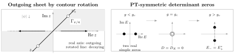
Complex boundary geometry selects the spectral sheet. Left: the outgoing inverted-oscillator solution on the real axis becomes Gaussian-decaying on the rotated contour $z=\ee^{\ii\pi/4}x$, with its two turning points on that contour. Right: two real zeros of a PT-symmetric determinant merge at $D=\partial_ED=0$ and continue as a conjugate pair. A contour rotation, a Stokes wall, and a determinant double zero are distinct operations.

PT symmetry constrains the zero set, not every zero

On a parity-symmetric contour, define

$$(\mathcal P\mathcal T\psi)(z) = \psi^*(-z^*).$$

The differential expression is PT symmetric when

$$V(-z^*;\mu)=V(z;\mu)^*$$

for real values of the declared couplings. The domain must also be invariant: parity and conjugation must exchange the two endpoint sectors or finite boundary lines.

If

$$H\psi=E\psi,$$

then anti-linearity gives

$$H(\mathcal P\mathcal T\psi) = E^*(\mathcal P\mathcal T\psi).$$

There are two possibilities.

• If a simple eigenfunction is also a PT eigenstate, then its eigenvalue is real. After a phase choice one can write $\mathcal P\mathcal T\psi=\psi$.

• If PT maps the eigenfunction to a linearly independent state, then $E$ and $E^*$ form a pair. The symmetry is often called broken on that pair.

PT symmetry therefore supplies a conjugation law for the determinant. With a suitable normalization it can be written

$$D(E^*;\mu)^*=D(E;\mu),$$

or the same equation multiplied by a nonzero analytic factor. It does not prove positivity, completeness, diagonalizability, or the existence of a positive metric. Those are separate spectral questions.

For polynomial problems at infinity, the domain condition is easy to miss. A potential may satisfy the pointwise PT relation while a chosen pair of decay wedges does not map into itself. That contour problem is not PT symmetric.

Why real spectra are nontrivial

The Bender–Boettcher family and related polynomial oscillators possess large regions with real spectra, and rigorous reality theorems are known for specified potentials and decay rays. The hypotheses include the boundary sectors. “The coefficients are PT symmetric” is not a substitute for such a theorem.

Exceptional points are determinant double zeros

Let $D(E,g)$ be analytic near a real point $(E_c,g_c)$ and suppose

$$\begin{aligned} D(E_c,g_c)&=0, & D_E(E_c,g_c)&=0, \\ D_{EE}(E_c,g_c)&\neq0, & D_g(E_c,g_c)&\neq0. \end{aligned}$$

Taylor expansion gives

$$0 = D_g\,\delta g +\frac12D_{EE}\,\delta E^2 +D_{Eg}\,\delta E\,\delta g +O\left(\delta E^3,\delta g^2\right),$$

where all displayed derivatives are evaluated at the critical point. Consequently,

$$\delta E^2 = -\frac{2D_g}{D_{EE}}\delta g +O\left(\delta g^{3/2}\right).$$

The two branches have a square-root Puiseux expansion. For a PT-symmetric one-parameter family, the coefficient can have the sign that produces two real roots on one side and a complex-conjugate pair on the other.

The equations $D=D_E=0$ detect an algebraic double zero. To call the point an exceptional point in the operator-theoretic sense, one also checks that the geometric multiplicity drops to one. In a scalar second-order problem with two separated boundary lines this is the generic outcome, but an ordinary semisimple degeneracy in a larger system must not be mislabeled.

The determinant is badly conditioned near the double zero because $D_E$ vanishes. Newton iteration in $E$ alone loses its usual quadratic model. Solve the augmented system

$$D(E,g)=0, \qquad D_E(E,g)=0$$

for $(E,g)$, or track both branches with a Puiseux parameter.

A solvable PT laboratory: the Airy box

Set $\hbar=1$ and consider

$$\begin{aligned} H_g\psi &= -\psi''+\ii g x\psi = E\psi, \\ \psi(-1)&=\psi(1)=0, \qquad g>0. \end{aligned}$$

The potential is not real, but $V(-x)^*=V(x)$ and the Dirichlet domain is PT invariant. Define the principal cube root

$$\alpha=(\ii g)^{1/3} = g^{1/3}\ee^{\ii\pi/6}$$

and the Airy coordinate

$$z(x;E,g) = \alpha \left( x+\frac{\ii E}{g} \right).$$

Because $\alpha^3=\ii g$,

$$\frac{\dd^2}{\dd x^2} \operatorname{Ai}(z) = (\ii gx-E)\operatorname{Ai}(z),$$

and similarly for $\operatorname{Bi}$. Put

$$z_\pm = \alpha \left( \pm1+\frac{\ii E}{g} \right).$$

The two endpoint equations have a nonzero common coefficient vector precisely when

$$\begin{aligned} D_{\mathrm A}(E,g) :={}& \operatorname{Ai}(z_-) \operatorname{Bi}(z_+) \\ &- \operatorname{Ai}(z_+) \operatorname{Bi}(z_-) =0. \end{aligned}$$

For $g>0$ and the declared cube-root branch,

$$\Delta_{\mathrm A}(E,g) := \ee^{-\ii\pi/6}D_{\mathrm A}(E,g)$$

is real when $E$ is real. Multiplying by this phase changes neither its zeros nor the ratio $-2D_g/D_{EE}$.

At $g=10$, the first two roots are

$$\begin{aligned} E_0&=4.5784904182916919\ldots, \\ E_1&=8.9966832557123482\ldots. \end{aligned}$$

They approach one another as $g$ grows. Solving the augmented Airy system gives the first collision

$$\begin{aligned} g_c &= 12.3124556722605251\ldots, \\ E_c &= 7.1085995967649488\ldots, \\ \Delta_{\mathrm A}(E_c,g_c) &= \partial_E\Delta_{\mathrm A}(E_c,g_c) =0. \end{aligned}$$

Numerically, $E_c/g_c=1/\sqrt3$ to the working precision. Direct differentiation of the determinant gives

$$-\frac{2\Delta_g}{\Delta_{EE}} = -2.3880593762328621\ldots.$$

Hence the local branches have the leading form

$$E_\pm(g) = E_c \pm 1.5453347133332837\ldots \sqrt{g_c-g} +O(g_c-g)$$

below the collision. Above it, the square root is imaginary and the pair leaves the real axis. For example, at $g=13$,

$$E_\pm = 7.2169577471438905\ldots \pm 1.3047650935833622\ldots\ii.$$

The only turning point is

$$x_t=-\frac{\ii E}{g}.$$

It remains simple at $(E_c,g_c)$. The exceptional point is therefore a global double zero of the endpoint determinant, not a turning-point collision. This is the promised concrete separation of two exceptional sets.

At fixed $g$, high eigenvalues satisfy

$$E_n \sim \frac{n^2\pi^2}{4}, \qquad n\to\infty,$$

because the kinetic term dominates on the finite interval. A finite difference matrix provides an independent check of the Airy determinant: below $g_c$ its lowest pair is real, while above $g_c$ the discretized matrix produces the same conjugate pair.

Conjugate actions make large order oscillate

Page 7 used a single positive action to produce a nearly fixed-sign factorial-over-power tail. Complex boundary problems often place the nearest Borel singularities at a conjugate pair

$$A=|A|\ee^{\ii\phi}, \qquad A^*=|A|\ee^{-\ii\phi}.$$

If their Stokes-weighted leading amplitudes are $C$ and $C^*$, their combined contribution has the form

$$\begin{aligned} a_n &\sim C\frac{\Gamma(n+\beta)}{A^{n+\beta}} + C^*\frac{\Gamma(n+\beta)}{(A^*)^{n+\beta}} \\ &= \frac{2|C|\Gamma(n+\beta)}{|A|^{n+\beta}} \cos\left[ \arg C-(n+\beta)\phi \right]. \end{aligned}$$

The envelope still reveals $|A|$, but the coefficients oscillate and a plain ratio $a_n/a_{n-1}$ need not converge. Phase-aware fits, Borel singularity plots, or short recurrences are better diagnostics. Whether both conjugate sectors enter with conjugate weights depends on the boundary problem and summation prescription; the potential alone does not decide it.

How complex turning points enter a practical WKB calculation

For a finite-interval PT problem, a straight endpoint path can miss the exponentially small term responsible for the interesting spectral structure. A leading one-turning-point calculation illustrates the mechanism. Let $x_t$ be the relevant complex turning point and define, in a convention with oscillatory momentum $p=\sqrt{E-V}$,

$$I_+ = \int_{x_t}^{1}p(x)\,\dd x.$$

PT symmetry relates the left integral to $I_+^*$. In the elementary Airy matching convention used by Bender and Jones, the leading secular equation takes the form

$$\sin\left(2\operatorname{Re}I_+\right) + \frac12 \exp\left(2\operatorname{Im}I_+\right) =0.$$

The exponential term is invisible to a direct no-turning-point rule. When it is small, the spectrum resembles the ordinary box. When it becomes comparable with the sine term, real roots can merge; after it is too large to balance a real sine, continuation to complex $E$ is required.

This equation is a leading WKB diagnostic, not the exact Airy determinant above and not a universal formula. For a pair of relevant turning points the matching equation changes. In exact WKB, the upgrade requires resummed open-path and cycle Voros symbols, the correct local connection matrices, and the chamber covariance of Page 5.

A safe workflow

1. Declare the domain. Record the spatial contour, endpoint sectors or finite boundary lines, time convention, and sheet of every asymptotic momentum.

2. Locate all turning points and singularities. Continue them as functions of $E$ and the couplings; do not select only the roots near the real axis by habit.

3. Draw the phased graph. Fix the Borel direction and determine which turning points actually connect the endpoint regions in the chosen chamber.

4. Choose relative paths and cycles. Record orientations, intersections, branch cuts, and any pole regularization.

5. Build boundary solutions. Use exact special functions where available; otherwise use Borel-summed WKB, numerical integration, or a controlled uniform approximation.

6. Form a determinant. Prefer a Wronskian or exterior product whose zeros are invariant under nonzero rescalings of the boundary solutions.

7. Search the correct sheet. For resonances, continue the outgoing momentum and compare with complex scaling or a scattering pole. For a PT problem, track conjugate branches together.

8. Classify singular events. Test separately for a curve discriminant, a Stokes wall, and $D=D_E=0$.

9. Demand independent checks. Vary base points, precision, contour angle, and discretization. A resonance should be stationary under an allowed scaling-angle change; an exceptional point should satisfy the augmented determinant system.

A reproducible audit

The companion checker instantiates every formula on this page. It performs the following independent tests:

• verifies the polynomial wedge spacing from the leading exponent;
• checks the inverted-oscillator contour rotation and Hermite residuals;
• compares a finite-difference complex-scaled oscillator with $E_n=-\ii(2n+1)$;
• evaluates the Airy determinant and its PT reality phase at high precision;
• solves $\Delta_{\mathrm A}=\partial_E\Delta_{\mathrm A}=0$ for the first exceptional point;
• checks the predicted square-root coefficient on both sides of the collision;
• compares Airy roots with an unrelated finite-difference matrix; and
• confirms conjugate pairing above the exceptional point.

The script reports its numerical tolerances and limitations. It does not prove dilation analyticity, Borel summability, completeness of resonant states, or the absence of additional spectral sheets.

Common pitfalls

Treating a complex contour as a plotting choice. The endpoint sectors and their subdominant lines define the operator domain. Crossing a sector boundary can replace a bound-state problem by a different non-Hermitian problem.

Calling every nonreal eigenvalue a resonance. A resonance is tied to an outgoing analytic continuation of a scattering problem. A complex eigenvalue of a finite PT-symmetric box is a genuine eigenvalue of that nonselfadjoint domain, not automatically a scattering pole.

Assuming PT symmetry implies reality. It implies that the spectral set is closed under complex conjugation when the domain is invariant. Reality requires an unbroken eigenstate or a stronger theorem.

Equating an exceptional point with coalescing turning points. The former is a multiple zero of a global determinant; the latter is a singularity of the local spectral curve. The Airy box has an exceptional point while its sole turning point stays simple.

Using complex scaling outside its analytic class. A stable-looking eigenvalue from one rotation angle is not enough. Check analyticity or use an admissible distortion, and test angle stationarity.

Forgetting the time sign. With $\ee^{-\ii Et/\hbar}$, decaying resonances lie in the lower half of the energy plane. Reversing the time factor reverses the naming of resonance and anti-resonance sheets.

Applying a real-axis WKB integral to a multivalued potential. The turning points and endpoints may lie on different sheets. A path that crosses a branch cut without recording the sheet change does not define the claimed action.

Exercises

1. Count the polynomial decay wedges

For $V(z)\sim az^m$, derive the boundary rays on which the two leading WKB exponentials have equal magnitude. Show that there are $m+2$ canonical sectors modulo $2\pi$.

Solution

Write

$$\chi(\phi) = \arg\sqrt a-\arg\hbar +\frac{m+2}{2}\phi.$$

Equal magnitude means $\cos\chi=0$, so

$$\phi_k = \frac{2}{m+2} \left[ \left(k+\frac12\right)\pi -\arg\sqrt a +\arg\hbar \right].$$

Adjacent rays are separated by $2\pi/(m+2)$. There are therefore $m+2$ sectors in one full turn. The subdominant sign alternates from sector to sector.

2. Recover the inverted-oscillator ladder

Apply $z=\ee^{\ii\pi/4}x$ to $H_{\mathrm{inv}}=-\hbar^2\partial_z^2-z^2$. Derive the resonance energies and verify that the analytically continued Gaussian is outgoing on both real ends.

Solution

The derivative and potential acquire the phases

$$-\hbar^2\partial_z^2 = -\ee^{-\ii\pi/2}\hbar^2\partial_x^2, \qquad -z^2=-\ee^{\ii\pi/2}x^2.$$

Thus $H_{\mathrm{inv}}=-\ii H_{\mathrm{osc}}$, and

$$E_n=-\ii\hbar(2n+1).$$

The rotated Gaussian becomes $\exp(\ii z^2/(2\hbar))$. Its phase derivative is $p=z$: momentum points right for $z>0$ and left for $z<0$, which is outgoing at both ends.

3. Prove determinant covariance

If the endpoint solutions are rescaled by nonzero analytic factors $f_j$ and $f_k$, show that the spectral zero divisor is unchanged. What quantity relevant to residues does change?

Solution

Bilinearity of the Wronskian gives

$$\widetilde D_{jk} = W[f_j\Psi_j,f_k\Psi_k] = f_jf_kD_{jk},$$

because $f_j$ and $f_k$ depend on spectral parameters, not on $z$. Their product is nonzero, so the zeros and their multiplicities are unchanged. At a simple zero $E_*$,

$$\widetilde D'(E_*) = f_j(E_*)f_k(E_*)D'(E_*),$$

so a residue proportional to $1/D'(E_*)$ changes unless the numerator and normalization are transformed consistently.

4. Derive PT conjugate pairing

Assume the potential and domain obey the PT conditions on this page. Show that a spectral point is either real or belongs to a conjugate pair. Why is a simple PT-invariant state real?

Solution

From $H\psi=E\psi$ and anti-linearity,

$$H(\mathcal P\mathcal T\psi) = E^*(\mathcal P\mathcal T\psi).$$

The transformed function obeys the same endpoint conditions, so $E^*$ is also spectral. If the eigenspace is one-dimensional and invariant, $\mathcal P\mathcal T\psi=c\psi$ for some nonzero $c$. Comparing the two eigenvalue equations gives $E=E^*$, hence $E$ is real.

5. Derive the exceptional-point square root

Starting from a double zero with $D_{EE}D_g\neq0$, derive the leading two spectral branches. State why this calculation alone does not prove the existence of a Jordan block.

Solution

Taylor expansion gives

$$D_g\delta g +\frac12D_{EE}\delta E^2 +O(\delta E\delta g,\delta E^3,\delta g^2) =0.$$

Since $\delta E=O(\delta g^{1/2})$,

$$E_\pm(g) = E_c \pm \sqrt{-\frac{2D_g}{D_{EE}}(g-g_c)} +O(g-g_c).$$

This describes the zero divisor of an analytic scalar function. A Jordan claim additionally concerns the geometric multiplicity and the domain of the operator pencil; those data are not contained in the Taylor series alone.

6. Build the Airy-box determinant

Starting from $-\psi''+\ii gx\psi=E\psi$, verify the Airy coordinate and derive $D_{\mathrm A}$ from the two Dirichlet equations.

Solution

Let $z=\alpha(x+\ii E/g)$ with $\alpha^3=\ii g$. For an Airy solution $u_{zz}=zu$,

$$u_{xx} = \alpha^2zu = \alpha^3 \left(x+\frac{\ii E}{g}\right)u = (\ii gx-E)u.$$

Hence

$$\psi=A\operatorname{Ai}(z)+B\operatorname{Bi}(z).$$

The two endpoint equations form the matrix

$$\begin{pmatrix} \operatorname{Ai}(z_-)&\operatorname{Bi}(z_-) \\ \operatorname{Ai}(z_+)&\operatorname{Bi}(z_+) \end{pmatrix} \begin{pmatrix}A\\B\end{pmatrix} =0.$$

Its determinant is exactly $D_{\mathrm A}$.

7. Fix the sign of a metastable width

Suppose

$$\mathcal Q_{\mathrm{well}}(E) +\ii cY=0,$$

where $c>0$, $Y>0$, and $\mathcal Q_{\mathrm{well}}'(E_0)>0$. Find the leading displacement of the simple real root $E_0$ and the sign of the width for $\ee^{-\ii Et/\hbar}$.

Solution

Set $E=E_0+\delta E$ and linearize:

$$\mathcal Q_{\mathrm{well}}'(E_0)\delta E +\ii cY=0.$$

Therefore

$$\delta E = -\ii \frac{cY}{\mathcal Q_{\mathrm{well}}'(E_0)}.$$

Writing $E=E_R-\ii\Gamma/2$ gives

$$\Gamma = \frac{2cY}{\mathcal Q_{\mathrm{well}}'(E_0)}>0.$$

The state decays in time. Reversing the radiation or time convention reverses the sign.

8. Sum a conjugate pair of large-order contributions

Starting with actions $A=|A|\ee^{\ii\phi}$ and $A^*$ and amplitudes $C=|C|\ee^{\ii\chi}$ and $C^*$, derive the oscillatory cosine law.

Solution

The first contribution is

$$\frac{|C|\Gamma(n+\beta)}{|A|^{n+\beta}} \ee^{\ii[\chi-(n+\beta)\phi]}.$$

The second is its complex conjugate. Their sum is

$$\frac{2|C|\Gamma(n+\beta)}{|A|^{n+\beta}} \cos\left[\chi-(n+\beta)\phi\right].$$

The cosine prevents an ordinary consecutive-coefficient ratio from approaching a single limit in general.

9. Classify the Airy-box collision

At the first Airy-box exceptional point, decide whether the spatial spectral curve is singular. Identify the calculation that detects the actual collision.

Solution

Here

$$R_0(x;E,g)=\ii gx-E, \qquad \partial_xR_0=\ii g.$$

Since $g_c\neq0$, the unique turning point is simple and the curve discriminant does not vanish. The spectral collision is instead detected by

$$D_{\mathrm A}(E_c,g_c)=0, \qquad \partial_ED_{\mathrm A}(E_c,g_c)=0.$$

It is a global degeneracy of the two-endpoint boundary problem.

From analytic determinants to controlled numbers

The output of this page is a declared analytic determinant on a declared complex sheet. Page 9 turns that object into controlled numbers. It develops Borel–Padé continuation on rotated and lateral rays, complex root tracking, argument-principle zero counts, precision escalation, and comparisons with direct Wronskian or matrix calculations.

References

• Sibuya, Y., Global Theory of a Second Order Linear Ordinary Differential Equation with a Polynomial Coefficient, North-Holland Mathematics Studies 18 (1975). The foundational global theory of canonical subdominant solutions and Stokes multipliers for polynomial equations.
• Voros, A., “The Return of the Quartic Oscillator: The Complex WKB Method”, Annales de l’Institut Henri Poincaré A 39 (1983), 211–338. Develops complex WKB, exact spectral functions, and global continuation for polynomial oscillators.
• Delabaere, E., and Pham, F., “Resurgent Methods in Semi-Classical Asymptotics”, Annales de l’Institut Henri Poincaré A 71 (1999), 1–94. Provides the resurgent exact-WKB framework behind chamber-dependent connection and spectral formulae.
• Delabaere, E., Dillinger, H., and Pham, F., “Exact Semiclassical Expansions for One-Dimensional Quantum Oscillators”, Journal of Mathematical Physics 38 (1997), 6126–6184. Treats resonance conditions as zeros of Jost symbols and derives the resurgent quantization and leading width of cubic shape resonances.
• Siegert, A. J. F., “On the Derivation of the Dispersion Formula for Nuclear Reactions”, Physical Review 56 (1939), 750–752. The historical source for purely outgoing, non-$L^2$ resonance states.
• Ramond, T., “Semiclassical Study of Quantum Scattering on the Line”, Communications in Mathematical Physics 177 (1996), 221–254. Gives a rigorous complex Bohr–Sommerfeld description of barrier-top resonances.
• Delabaere, E., and Pham, F., “Eigenvalues of Complex Hamiltonians with PT-Symmetry. I” and Part II, Physics Letters A 250 (1998). Uses complex WKB and exact model quantization conditions to analyze reality domains and pairwise level coalescence.
• Aguilar, J., and Combes, J. M., “A Class of Analytic Perturbations for One-Body Schrödinger Hamiltonians”, Communications in Mathematical Physics 22 (1971), 269–279, and Balslev, E., and Combes, J. M., “Spectral Properties of Many-Body Schrödinger Operators with Dilatation-Analytic Interactions”, 22 (1971), 280–294. Foundational complex-scaling theorems.
• Zworski, M., “Mathematical Study of Scattering Resonances”, Bulletin of Mathematical Sciences 7 (2017), 1–85. Reviews resolvent resonances, outgoing states, complex scaling, and the operator-theoretic hypotheses connecting them.
• Bender, C. M., and Boettcher, S., “Real Spectra in Non-Hermitian Hamiltonians Having PT Symmetry”, Physical Review Letters 80 (1998), 5243–5246. Introduces the polynomial PT-symmetric spectral families and their complex decay wedges.
• Shin, K. C., “On the Reality of the Eigenvalues for a Class of PT-Symmetric Oscillators”, Communications in Mathematical Physics 229 (2002), 543–564, and Dorey, P., Dunning, C., and Tateo, R., “Spectral Equivalences, Bethe Ansatz Equations, and Reality Properties in PT-Symmetric Quantum Mechanics”, Journal of Physics A 34 (2001), 5679–5704. Prove reality only for specified polynomial families and boundary rays.
• Ahmed, Z., “Eigenvalue Problems for the Complex PT-Symmetric Potential $V(x)=igx$”, Physics Letters A 364 (2007), 12–16. Gives the Airy hard-box determinant and its exceptional-point spectrum.
• Bender, C. M., and Jones, H. F., “WKB Analysis of PT-Symmetric Sturm–Liouville Problems”, Journal of Physics A 45 (2012), 444004, and Part II, Physical Review A 85 (2012), 052118. Derive one- and two-turning-point secular equations and test their exceptional-point predictions.
• Kato, T., Perturbation Theory for Linear Operators, Springer (1995 reprint). Supplies the analytic-operator framework for eigenvalue branching, algebraic multiplicity, and exceptional points.
• NIST Digital Library of Mathematical Functions, §12.2, especially the parabolic-cylinder Wronskian identity. Calibrates the outgoing and incoming inverted-Weber determinants used above.