Analyticity Strips, Kernels, Driving Terms, and Contours

Page 1 listed the analytic passport needed to invert a functional relation. This page performs the inversion for two ground-state passports. A truncated fused $Y$-system produces a matrix Green function on a finite graph; a $TQ$ auxiliary ratio produces a one-function DDV equation from a keyhole contour around a selected root divisor.

The calculations share a rapidity coordinate and a WKB scale, but they do not share a shift, kernel, or contour. The most visible consequence is a factor of two:

$$\begin{array}{c|c|c} \text{route} & \text{multiplicative shift} & \text{first rapidity half-strip} \\ \hline \text{fused }Y\text{-system} & q^{\pm1}s & \pi/(2M) \\ \text{DDV auxiliary ratio} & q^{\pm2}s & \pi/M \end{array}$$

All formulae below are ground-state, first-strip formulae. Contour crossings, excited roots, holes, and wall crossing belong to Page 5.

Status ledger

Passage	Status on this page
Fourier multiplier for a strip-boundary shift	Exact under the stated Hardy and boundary hypotheses
Absence of residue terms during a contour shift	A ground-state analytic assumption, checked against the declared divisor
Growing drive as a homogeneous mode	Exact algebraically; its coefficient is fixed by ODE/WKB asymptotics
Negative-rapidity stationary constants	Exact stationary $Y$-system solution; the positive branch is selected by the ground-state passport
Finite-graph matrix inverse	Exact finite-dimensional Fourier algebra
Fused-node TBA	Exact representation under truncation, ANZC, branch, endpoint, and contour hypotheses
Cauchy replacement of the TQ root sum	Exact for the selected simple divisor and the declared keyhole contour
DDV kernel, bare twist, and drive	Exact in the primary Dorey–Tateo convention
Existence or uniqueness of a general nonlinear solution	Not claimed; numerical convergence is treated on Page 6
Exact-WKB/GMN kernel	A different Riemann–Hilbert construction, introduced on Page 3

A strip is more than an open domain

For $\eta>0$, write

$$S_\eta = \{\theta\in\mathbb C:|\Im\theta|<\eta\}.$$

Four logically distinct statements are often compressed into the phrase “analytic in the strip”:

1. the function is holomorphic in the open set $S_\eta$;
2. every argument of a chosen logarithm is nonzero there;
3. controlled boundary traces exist on $\mathbb R\pm\ii\eta$;
4. the vertical sides of a closing rectangle make no contribution.

Entirety in $s$ proves none of the last three after the exponential pullback $s=s_\star\exp(\theta/\rho_M)$. The pullback can have repeated images of zeros, and the boundary lines can pass through them.

Here is the contour-shift lemma used in both routes. Let $g$ be holomorphic in $S_\eta$, admit $L^1$ boundary traces, and obey

$$\sup_{|y|<\eta} \int_{\mathbb R}|g(x+\ii y)|\,\dd x<\infty.$$

Assume also that the vertical-edge integrals vanish as the closing rectangle expands. With the Fourier convention of Page 1,

$$\widehat g(k) = \int_{\mathbb R}\ee^{\ii kx}g(x)\,\dd x,$$

Cauchy’s theorem gives

$$\begin{aligned} \widehat{g(\,\cdot+\ii\eta\,)}(k) &=\ee^{\eta k}\widehat g(k), \\ \widehat{g(\,\cdot-\ii\eta\,)}(k) &=\ee^{-\eta k}\widehat g(k). \end{aligned}$$

The signs can be checked by putting $z=x+\ii\eta$, so that $\ee^{\ii kx}=\ee^{\eta k}\ee^{\ii kz}$. If a pole, zero-induced logarithmic cut, or kernel singularity lies between the two contours, Cauchy’s theorem adds a residue or jump term. That is the mechanism behind the sources deferred to Page 5.

The growing and constant endpoints need different treatments

For the finite $A_{h-1}$ system, define the logarithmic difference operator

$$(\mathcal D u)_a(\theta) = u_a\!\left(\theta+\frac{\pi\ii}{h}\right) +u_a\!\left(\theta-\frac{\pi\ii}{h}\right) -\sum_b I_{ab}u_b(\theta).$$

On the ground-state branch,

$$\mathcal D\varepsilon=I L, \qquad L_a=\log(1+\ee^{-\varepsilon_a}).$$

There are two obstructions to an ordinary Fourier transform. At positive rapidity,

$$d_a(\theta) =\mathfrak m_a\ee^\theta, \qquad \mathcal Dd=0,$$

grows exponentially. At negative rapidity,

$$\varepsilon_a(\theta)\longrightarrow c_a, \qquad L_a(\theta)\longrightarrow \ell_a,$$

so neither remainder is generally integrable. The stationary relation is

$$\sum_b \bigl(2\delta_{ab}-I_{ab}\bigr)c_b = \sum_b I_{ab}\ell_b.$$

A switching function makes the endpoint bookkeeping explicit. Choose $\chi$ analytic in the working strip, with $\chi\to1$ at $-\infty$ and $\chi\to0$ at $+\infty$. For example,

$$\chi(\theta)=\frac{1}{1+\ee^{\sigma\theta}}, \qquad 0<\sigma<\frac{\pi}{\eta},$$

keeps its nearest poles outside $S_\eta$. Set

$$\begin{aligned} g_a&=\varepsilon_a-d_a-c_a\chi, \\ r_a&=L_a-\ell_a\chi. \end{aligned}$$

Then $g$ and $r$ decay at both ends, while

$$\mathcal Dg = I r+S^\chi,$$

with the localized switching source

$$S_a^\chi(\theta) = c_a\!\left[ 2\chi(\theta) -\chi\!\left(\theta+\frac{\pi\ii}{h}\right) -\chi\!\left(\theta-\frac{\pi\ii}{h}\right) \right].$$

This source is not an excited-state source. It is a regulator term whose sole job is to restore the negative-end constant. Reconstructing $\varepsilon$ cancels the choice of $\chi$. Equivalently, one may use the exponentially regulated Fourier transform of Dorey–Dunning–Tateo or work with tempered distributions, retaining the full distributional endpoint contribution at zero momentum.

Finite fusion produces a matrix Green function

For the polynomial subclass used here, take $l=0$, $M\in\mathbb Z$, $M>1$, and $h=2M$. Put

$$x=\frac{\pi k}{h}.$$

Assume that the regulated remainders $g$, $r$, and $S^\chi$ satisfy the strip-boundary, Hardy, and vanishing-vertical-edge hypotheses stated above, with no intervening divisor. Under these hypotheses, Fourier transformation of the regulated equation introduces

$$\mathcal A_{ab}(k) = 2\cosh x\,\delta_{ab}-I_{ab}.$$

The orthonormal sine vectors

$$v_a^{(r)} = \sqrt{\frac2h} \sin\!\left(\frac{\pi r a}{h}\right), \qquad r=1,\ldots,h-1,$$

diagonalize the incidence matrix:

$$\sum_b I_{ab}v_b^{(r)} = 2\cos\!\left(\frac{\pi r}{h}\right)v_a^{(r)}.$$

Therefore $\mathcal A(k)$ is invertible for every real $k$. Its inverse has the useful closed form

$$\begin{aligned} \bigl[\mathcal A(k)^{-1}\bigr]_{ab} ={}& \frac{ \sinh(a_<x)\sinh((h-a_>)x) }{ \sinh x\,\sinh(hx) }, \\ a_<&=\min(a,b), \qquad a_>=\max(a,b). \end{aligned}$$

At $k=0$, this is understood by continuity:

$$\bigl[\mathcal A(0)^{-1}\bigr]_{ab} = \frac{a_<(h-a_>)}{h}.$$

Define the matrix convolution kernel by

$$\widehat{\mathsf K}(k) = \mathcal A(k)^{-1}I.$$

If one prefers the scattering-kernel convention, set $\widehat\phi=-2\pi\widehat{\mathsf K}$. The two identical forms of the ground-state massless TBA are then

$$\begin{aligned} \varepsilon_a(\theta) ={}&d_a(\theta) +\sum_b \int_{\mathbb R} \mathsf K_{ab}(\theta-\theta')L_b(\theta')\,\dd\theta' \\ ={}&d_a(\theta) -\frac{1}{2\pi} \sum_b \int_{\mathbb R} \phi_{ab}(\theta-\theta')L_b(\theta')\,\dd\theta'. \end{aligned}$$

The bounded convolution includes the left endpoint because

$$c=\widehat{\mathsf K}(0)\ell.$$

Thus the switching construction and the distributional construction give the same result. The slowest-decaying entries of $\widehat{\mathsf K}(k)$ are $O(\ee^{-\pi|k|/h})$ as $|k|\to\infty$, so the direct kernel representation has first half-strip $\pi/h$.

ODE asymptotics fix the massless drive

Return to the Chapter 12 normalization

$$\rho_M=\frac{M+1}{2M}, \qquad s=v_ME, \qquad \theta=\rho_M\Log\!\left(\frac{s}{s_\star}\right).$$

Define the positive WKB coefficient

$$b_0 = \frac{ \sqrt\pi\,\Gamma(\frac{1}{2M}) }{ M\,\Gamma(\frac32+\frac{1}{2M}) },$$

and two rapidity-scale coefficients

$$\begin{aligned} \mathfrak m_{\mathrm D}(s_\star) &= \frac{b_0}{2} \left(\frac{s_\star}{v_M}\right)^{\rho_M}, \\ \mathfrak m_{\mathrm Y}(s_\star) &= b_0 \left(\frac{s_\star}{v_M}\right)^{\rho_M} =2\mathfrak m_{\mathrm D}(s_\star). \end{aligned}$$

The factor of two follows directly from the centered fused asymptotic. For $1\le n\le h-1$,

$$\log T_{n/2}(s) \sim \frac{b_0}{ 2\cos(\frac{\pi}{h})v_M^{\rho_M} } \sin\!\left(\frac{\pi n}{h}\right)s^{\rho_M}.$$

At $n=0,h$, the same leading formula holds trivially because $T_0=T_{h/2}=1$ and the sine vanishes.

Since $Y_a=T_{(a-1)/2}T_{(a+1)/2}$, the addition formula gives

$$\begin{aligned} \log Y_a(s) &\sim \frac{b_0}{v_M^{\rho_M}} \sin\!\left(\frac{\pi a}{h}\right)s^{\rho_M} \\ &= \mathfrak m_{\mathrm Y}(s_\star) \sin\!\left(\frac{\pi a}{h}\right)\ee^\theta. \end{aligned}$$

The fused-node drive is

$$d_a(\theta) = \mathfrak m_{\mathrm Y}(s_\star) \sin\!\left(\frac{\pi a}{h}\right)\ee^\theta.$$

This is the Perron–Frobenius vector required by the homogeneous difference equation. Its absolute coefficient is not obtained from the $Y$-system: it is the leading ODE determinant asymptotic expressed in the chosen rapidity origin. The fused $Y_a$ contains a product of two neighboring transfer functions, whereas the DDV auxiliary function contains one radial determinant ratio. If $s_\star\mapsto\lambda s_\star$, then $\theta\mapsto\theta-\rho_M\log\lambda$ and both coefficients acquire the factor $\lambda^{\rho_M}$. Hence both $\mathfrak m_{\mathrm D}(s_\star)\ee^\theta$ and $\mathfrak m_{\mathrm Y}(s_\star)\ee^\theta$ are unchanged. This is why a formula written with an independently shifted massless rapidity—as in Appendix E.1 of the 2007 review—can display a different bare coefficient until its rapidity origin is mapped to the present $s_\star$ convention.

The positive stationary solution at the other endpoint is

$$\mathcal Y_a = \frac{ \sin(\frac{\pi a}{h+2}) \sin(\frac{\pi(a+2)}{h+2}) }{ \sin^2(\frac{\pi}{h+2}) },$$

with

$$c_a=\log\mathcal Y_a, \qquad \ell_a=\log(1+\mathcal Y_a^{-1}).$$

For the quartic oscillator, $M=2$ and $h=4$. The drive ratios and stationary values are

$$\begin{aligned} (\mathfrak m_1,\mathfrak m_2,\mathfrak m_3) &\propto(1,\sqrt2,1), \\ (\mathcal Y_1,\mathcal Y_2,\mathcal Y_3) &=(2,3,2). \end{aligned}$$

This is the three-node $A_3$ problem, not the scalar calibration of Page 1.

A keyhole contour selects the radial TQ divisor

For the regular radial determinant, work in the clean window

$$M>1, \qquad -\frac12<l<\frac M2.$$

The normalized $Q_+$ has positive simple zeros $s_n$, while the associated transfer zeros lie on the negative axis. The second statement uses the PT-symmetric positivity theorem in the 2001 Dorey–Dunning–Tateo paper cited below; it is not a consequence of the $TQ$ identity alone. With

$$a(s) = \ee^{2\ii\vartheta} \frac{Q_+(q^2s)}{Q_+(q^{-2}s)},$$

the genus-zero product gives

$$\Log a(s) = 2\ii\vartheta +\sum_{n=0}^{\infty} F\!\left(\frac{s}{s_n}\right),$$

where

$$F(z) = \Log\!\left(\frac{1-q^2z}{1-q^{-2}z}\right).$$

Let $\mathcal C$ be a counterclockwise keyhole around the positive axis: its upper lip runs from $+\infty$ to the origin and its lower lip returns to $+\infty$. It encloses the radial zeros of $1+a$, but not the negative transfer zeros or poles of the shifted denominator. The argument principle gives

$$\begin{aligned} \Log a(s) ={}&2\ii\vartheta \\ &+ \oint_{\mathcal C} \frac{\dd s'}{2\pi\ii}\, F\!\left(\frac{s}{s'}\right) \partial_{s'}\Log(1+a(s')). \end{aligned}$$

One can first prove this identity for a finite determinant and then take the canonical-product limit uniformly on compact subsets avoiding the divisor. The small circle around the origin and the large closing arc must vanish in that limit; neither disappearance follows from a formal root sum alone.

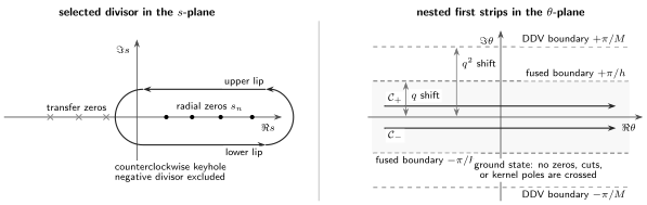
Ground-state residue-free geometries. The keyhole selects the radial divisor before it becomes the two rapidity contours $\mathcal C_\pm$. The fused TBA reaches the $q$-shift boundaries $|\Im\theta|=\pi/(2M)$; the direct DDV equation reaches the $q^2$ boundaries $|\Im\theta|=\pi/M$. A zero, cut, or kernel pole crossing any displayed contour changes the integral equation.

Wiener–Hopf inversion gives the primary-sign DDV equation

Write

$$s=s_\star\exp\!\left(\frac{\theta}{\rho_M}\right), \qquad f(\theta)=\Log a(s).$$

The two lips of the keyhole become contours $\mathcal C_-=\mathbb R-\ii0$ and $\mathcal C_+=\mathbb R+\ii0$, both oriented from left to right after integration by parts. Matching the WKB asymptotic and fixing the continuous ground-state branch gives

$$\begin{aligned} f(\theta) ={}& \ii\pi\!\left(l+\frac12\right) -\ii\mathfrak m_{\mathrm D}(s_\star)\ee^\theta \\ &+ \int_{\mathcal C_-} G_M(\theta-\theta') \Log(1+\ee^{f(\theta')})\,\dd\theta' \\ &- \int_{\mathcal C_+} G_M(\theta-\theta') \Log(1+\ee^{-f(\theta')})\,\dd\theta'. \end{aligned}$$

In the convention of the original Dorey–Tateo derivation,

$$\begin{aligned} G_M(\theta) &= \int_{\mathbb R}\frac{\dd k}{2\pi}\, \ee^{-\ii k\theta}\widehat G_M(k), \\ \widehat G_M(k) &= \frac{ \sinh[ \frac{\pi k}{2}(\frac1M-1) ] }{ 2\cosh(\frac{\pi k}{2}) \sinh(\frac{\pi k}{2M}) }. \end{aligned}$$

For $M>1$ this is the negative-sign kernel. In particular,

$$\widehat G_M(0)=\frac{1-M}{2},$$

and the quartic specialization is

$$G_2(\theta) = -\frac{1}{2\pi\cosh\theta}.$$

Do not splice kernel conventions

The 1999 primary equation for the auxiliary ratio defined above has the numerator $(1/M-1)$. In the 2007 review, D.55 instead defines the positive kernel $\Phi_M=-G_M$, consistently with the real-axis equation D.51, but D.56 does not reverse the two signs on returning to contour form. This page is normalized to the primary equation; replacing $G_M$ by $-G_M$ without changing the surrounding equation fails the endpoint check below.

The bare constant $\ii\pi(l+\tfrac12)$ is not $f(-\infty)$. Put

$$\alpha = \frac{\pi(2l+1)}{M+1} =2\vartheta.$$

Since $a(0)=\ee^{\ii\alpha}$ and $0<\alpha<\pi$ in the clean window,

$$\begin{aligned} &\Log(1+\ee^{\ii\alpha}) -\Log(1+\ee^{-\ii\alpha}) =\ii\alpha, \\ &\ii\pi\!\left(l+\frac12\right) +\widehat G_M(0)\,\ii\alpha =\ii\alpha. \end{aligned}$$

Thus the convolution restores the exact small-$s$ twist. This one-line calibration fixes both the kernel sign and its zero-momentum normalization.

On the real axis, Schwarz reflection combines the two lips. With $Z=\ii f$, the real counting equation is

$$\begin{aligned} Z(\theta) ={}& -\pi\!\left(l+\frac12\right) +\mathfrak m_{\mathrm D}(s_\star)\ee^\theta \\ &- 2\int_{\mathbb R} G_M(\theta-\theta') \Im\Log(1+a(\theta'-\ii0))\,\dd\theta'. \end{aligned}$$

The radial levels obey

$$Z(\theta_n)=(2n+1)\pi, \qquad E_n = \frac{s_\star}{v_M} \exp\!\left(\frac{\theta_n}{\rho_M}\right),$$

with the integer ordering fixed by the continuous branch and the Weyl asymptotic.

The two first strips must not be interchanged

The DDV multiplier decays as $\ee^{-\pi|k|/M}$. Its direct convolution is analytic only for

$$|\Im\theta| < \min\!\left(\pi,\frac{\pi}{M}\right) =\frac{\pi}{M}, \qquad M>1.$$

The first kernel poles occur at $\theta=\pm\pi\ii/M$. A second generic singularity scale is $\theta=\pm\pi\ii$, although special values of $M$ can cancel individual poles; for example, $G_2=-1/(2\pi\cosh\theta)$ has no pole at $\pm\pi\ii$. Continuing through the first pair requires a second determination and an added residue term. The upper bank of the negative $s$-axis maps to

$$\Im\theta = \pi\rho_M = \frac{\pi(M+1)}{2M},$$

while the lower bank maps to the reflected line $\Im\theta=-\pi\rho_M$.

Both banks lie outside the first DDV strip for $M>1$. Lateral levels therefore cannot be obtained by direct substitution into the first-strip equation.

For the finite fused system, the matrix kernel instead has first half-strip $\pi/h=\pi/(2M)$. Its unknowns, divisor data, and endpoint constants are different:

Feature	TQ/DDV route	Fused-node TBA
Shift	$q^{\pm2}s$	$q^{\pm1}s$
Unknown	one complex $a$ or $Z$	$h-1$ node pseudoenergies
Contour	two lips around the selected radial ray	shifted strip boundaries reduced to the real line
Kernel	scalar Cauchy/Wiener–Hopf inverse $G_M$	matrix inverse $\mathcal A^{-1}I$
Drive	bare twist plus $-\ii\mathfrak m_{\mathrm D}\ee^\theta$	Perron–Frobenius vector times $\mathfrak m_{\mathrm Y}\ee^\theta$, with $\mathfrak m_{\mathrm Y}=2\mathfrak m_{\mathrm D}$
Finite closure	not required	required
First half-strip	$\pi/M$	$\pi/(2M)$

Neither kernel is an exact-WKB/GMN kernel. There the discrete input is an intersection pairing and a set of BPS rays, not a Baxter divisor or a Dynkin incidence matrix.

Ground-state contours stop before source terms

Every displayed equation on this page assumes:

• no zero or hole crosses $\mathcal C_\pm$;
• no zero of $Y_a$ or $1+Y_a$ crosses a shifted strip boundary;
• no logarithmic cut is dragged through an integration contour;
• no kernel pole is crossed during analytic continuation;
• the branch integers remain those of the ground-state passport.

When one of these conditions fails, the correct response is not to continue the same formula numerically. The contour must be deformed, the crossed residues must be recorded, and new root conditions may have to be solved simultaneously. Page 5 carries out that calculation.

Common pitfalls

Equating open-strip holomorphy with boundary control. A contour shift needs boundary traces and vanishing vertical sides. Holomorphy in the open strip alone supplies neither.

Fourier transforming both endpoints naively. The WKB drive grows at $+\infty$, while the stationary solution is nonzero at $-\infty$. They require a homogeneous subtraction and a zero-momentum regulator, respectively.

Using one strip width for both routes. The fused system shifts by $q$, while the auxiliary ratio shifts by $q^2$. Their half-strips differ by a factor of two.

Copying a kernel without its auxiliary-function definition. The changes $a\mapsto a^{-1}$ and $G\mapsto-G$ alter twists, drives, and contour signs together. The quartic and small-$s$ checks detect an inconsistent splice.

Calling the DDV keyhole a TBA contour. It surrounds a selected root divisor. The fused TBA instead inverts boundary values of a finite node system.

Substituting a lateral level into the first strip. The negative spectral ray lies beyond the first DDV kernel pole. A second determination is required.

Exercises

1. Prove the strip-shift multipliers

Let $g$ satisfy the strip hypotheses stated on this page. Prove

$$\widehat{g(\,\cdot\pm\ii\eta\,)}(k) = \ee^{\pm\eta k}\widehat g(k)$$

by closing a rectangle. Identify exactly where the proof fails if a simple pole lies between the contours.

Solution

For the upper shift, put $z=x+\ii\eta$. Then

$$\begin{aligned} \int_{\mathbb R}\ee^{\ii kx}g(x+\ii\eta)\,\dd x &= \ee^{\eta k} \int_{\mathbb R+\ii\eta} \ee^{\ii kz}g(z)\,\dd z. \end{aligned}$$

Close the rectangle with horizontal sides $\mathbb R$ and $\mathbb R+\ii\eta$. The assumed vertical-edge decay and absence of singularities let the upper integral move to the real axis, giving $\ee^{\eta k}\widehat g(k)$. Repeating the argument in the lower half-strip gives $\ee^{-\eta k}\widehat g(k)$.

If a pole $z_0$ is crossed, the rectangle encloses it and the two horizontal integrals differ by

$$2\pi\ii\, \operatorname*{Res}_{z=z_0} \bigl(\ee^{\ii kz}g(z)\bigr),$$

with a sign fixed by the direction of displacement. The pure multiplier identity is then false; the residue becomes a source after inverse transformation.

2. Derive the switching source

Starting from $\mathcal D\varepsilon=I L$ and $(2\mathbf1-I)c=I\ell$, derive $S^\chi$. Then show algebraically that changing $\chi$ cannot change the reconstructed pseudoenergy.

Solution

Since $\mathcal Dd=0$,

$$\mathcal Dg = I L-\mathcal D(c\chi).$$

Subtract and add $I\ell\chi$:

$$\mathcal Dg = I(L-\ell\chi) +I\ell\chi-\mathcal D(c\chi).$$

Using $I\ell=(2\mathbf1-I)c$, the last two terms reduce componentwise to

$$S_a^\chi = c_a(2\chi-\chi^+-\chi^-).$$

Now let $\delta\chi=\chi_1-\chi_2$. The two decompositions have

$$\delta g=-c\,\delta\chi, \qquad \delta r=-\ell\,\delta\chi, \qquad \delta S =c(2\delta\chi-\delta\chi^+-\delta\chi^-).$$

Direct substitution gives $\mathcal D(\delta g)=I\delta r+\delta S$. Thus the change in the Fourier-inverted remainder is exactly $-c\,\delta\chi$; adding back $c\chi$ cancels it. The reconstructed $\varepsilon$ is independent of the regulator.

3. Diagonalize the finite-graph multiplier

Using the sine vectors $v^{(r)}$, find every eigenvalue of $\mathcal A(k)$ and prove real-$k$ invertibility. Derive a spectral-sum formula for its inverse.

Solution

The incidence eigenvalue on $v^{(r)}$ is $2\cos(\pi r/h)$. Therefore

$$\lambda_r(k) = 2\cosh\!\left(\frac{\pi k}{h}\right) -2\cos\!\left(\frac{\pi r}{h}\right).$$

For real $k$ and $1\le r\le h-1$, one has $\cosh(\pi k/h)\ge1$ and $\cos(\pi r/h)<1$. Hence $\lambda_r(k)>0$ and $\mathcal A(k)$ is invertible. Completeness of the orthonormal sine basis gives

$$\bigl[\mathcal A(k)^{-1}\bigr]_{ab} = \frac2h \sum_{r=1}^{h-1} \frac{ \sin(\frac{\pi r a}{h}) \sin(\frac{\pi r b}{h}) }{ 2\cosh(\frac{\pi k}{h}) -2\cos(\frac{\pi r}{h}) }.$$

Summing this finite Green function yields the hyperbolic-sine form in the text.

4. Verify the stationary A-type solution

Let $t=\pi/(h+2)$ and

$$\mathcal Y_a = \frac{\sin(at)\sin((a+2)t)}{\sin^2t}.$$

Prove the constant $A_{h-1}$ $Y$-system and then recover $(2\mathbf1-I)c=I\ell$.

Solution

The elementary identity

$$\sin^2((a+1)t) -\sin(at)\sin((a+2)t) =\sin^2t$$

implies

$$1+\mathcal Y_a = \frac{\sin^2((a+1)t)}{\sin^2t}.$$

With $\mathcal Y_0=\mathcal Y_h=0$,

$$\mathcal Y_a^2 =(1+\mathcal Y_{a-1})(1+\mathcal Y_{a+1}),$$

because both sides equal $\sin^2(at)\sin^2((a+2)t)/\sin^4t$.

Take logarithms and use

$$\log(1+\mathcal Y_b) =c_b+\ell_b.$$

The constant $Y$-system becomes $2c_a=\sum_bI_{ab}(c_b+\ell_b)$, which rearranges to $(2\mathbf1-I)c=I\ell$.

5. Calibrate the quartic A₃ matrix

For $M=2$, write $\mathcal A(k)$ explicitly, list its three eigenvalues, and verify the node drive ratio, the relation between the fused and DDV drive scales, and the negative-end constant equation.

Solution

Put $x=\pi k/4$. Then

$$\mathcal A(k) = \begin{pmatrix} 2\cosh x&-1&0\\ -1&2\cosh x&-1\\ 0&-1&2\cosh x \end{pmatrix}.$$

The incidence eigenvalues are $\sqrt2,0,-\sqrt2$, so the three $\mathcal A$ eigenvalues are

$$2\cosh x-\sqrt2, \qquad 2\cosh x, \qquad 2\cosh x+\sqrt2.$$

The Perron–Frobenius vector has components $\sin(a\pi/4)$, hence ratio $(1,\sqrt2,1)$. The matrix fixes only this ratio. Invoking the large-$s$ fused asymptotic derived above fixes the absolute comparison and gives

$$\mathfrak m_{\mathrm Y} =2\mathfrak m_{\mathrm D}, \qquad d_2(\theta) =\mathfrak m_{\mathrm Y}\ee^\theta =2\mathfrak m_{\mathrm D}\ee^\theta.$$

Thus the middle fused node carries twice the magnitude of the DDV WKB coefficient before the DDV phase $-\ii$ is included.

At negative rapidity,

$$c=(\log2,\log3,\log2), \qquad \ell= \left( \log\frac32, \log\frac43, \log\frac32 \right).$$

Using the $A_3$ incidence matrix,

$$(2\mathbf1-I)c = \left( \log\frac43, \log\frac94, \log\frac43 \right) =I\ell.$$

This checks both endpoint normalization and node ordering.

6. Calibrate the keyhole orientation

Suppose a holomorphic function $H(s')$ has exactly two simple zeros $u$ and $v$ inside a counterclockwise keyhole and no poles there. Assume $F(s/s')$ is analytic on and inside the contour. Evaluate

$$\oint_{\mathcal C} \frac{\dd s'}{2\pi\ii}\, F\!\left(\frac{s}{s'}\right) \partial_{s'}\Log H(s').$$

Solution

Near a simple zero $u$,

$$\partial_{s'}\Log H(s') =\frac{1}{s'-u}+\text{holomorphic},$$

and similarly at $v$. The two residues are therefore $F(s/u)$ and $F(s/v)$. Counterclockwise orientation gives

$$\oint_{\mathcal C} \frac{\dd s'}{2\pi\ii}\, F\!\left(\frac{s}{s'}\right) \partial_{s'}\Log H(s') =F\!\left(\frac{s}{u}\right) +F\!\left(\frac{s}{v}\right).$$

Reversing the keyhole would negate the root sum. Extra zeros of $1+a$ or poles of the shifted denominator would add their own signed residues, which is why the divisor passport is indispensable.

7. Keep the two DDV sign packages coherent

Define $\Phi_M=-G_M$, so that $\widehat\Phi_M(k)>0$ for every real $k$ when $M>1$. Rewrite the DDV contour terms using $\Phi_M$. Explain why changing only the kernel sign is inconsistent.

Solution

The primary-sign package is

$$+\int_{\mathcal C_-}G_M L_- -\int_{\mathcal C_+}G_M L_+.$$

Since $\Phi_M=-G_M$, the identical expression is

$$-\int_{\mathcal C_-}\Phi_M L_- +\int_{\mathcal C_+}\Phi_M L_+.$$

Thus a positive kernel requires the lower and upper contour signs to reverse together. If one inserts $\Phi_M$ but retains $+\mathcal C_- -\mathcal C_+$, the zero-momentum mass changes from $(1-M)/2$ to $(M-1)/2$. The small-$s$ endpoint then no longer returns $f(-\infty)=2\ii\vartheta$. Kernel sign, contour signs, and the definition of $a$ form one convention package.

8. Locate the two strip boundaries

Use the large-$|k|$ behavior of the two Fourier kernels to find their direct half-strips. Specialize to $M=2$ and locate the negative spectral ray in the rapidity plane.

Solution

For the finite-node kernel,

$$\widehat{\mathsf K}(k) =O\!\left(\ee^{-\pi|k|/h}\right),$$

so its inverse transform is directly analytic for $|\Im\theta|<\pi/h$. With $h=2M$, this is $\pi/(2M)$.

For DDV,

$$\widehat G_M(k) =O\!\left(\ee^{-\pi|k|/M}\right),$$

so the direct half-strip is $\pi/M$ for $M>1$. At $M=2$, the fused and DDV half-widths are respectively $\pi/4$ and $\pi/2$.

The upper bank of the negative $s$-axis has

$$\Im\theta =\pi\rho_2 =\frac{3\pi}{4}.$$

The lower bank lies at $-3\pi/4$. Both lie beyond the first DDV poles at $\pm\pi/2$, and therefore also beyond the fused strip. Reaching them in the DDV representation requires the appropriate second determination. The fused representation likewise requires analytic continuation with the crossed residues, or equivalently suitable shifted $Y$-system relations. Direct substitution into either first-strip formula is invalid.

References

• V. V. Bazhanov, S. L. Lukyanov, and A. B. Zamolodchikov, “Integrable Structure of Conformal Field Theory II. Q-Operator and DDV Equation,” Communications in Mathematical Physics 190 (1997), 247–278, arXiv:hep-th/9604044, doi:10.1007/s002200050240. Section 3 and Appendix A derive the auxiliary-function inversion, its asymptotic zero mode, and the DDV kernel under explicit analytic assumptions.
• C. Destri and H. J. de Vega, “New Thermodynamic Bethe Ansatz Equations without Strings,” Physical Review Letters 69 (1992), 2313–2317, doi:10.1103/PhysRevLett.69.2313. The original nonlinear-integral-equation framework behind the one-function counting equation.
• P. Dorey and R. Tateo, “Anharmonic Oscillators, the Thermodynamic Bethe Ansatz, and Nonlinear Integral Equations,” Journal of Physics A 32 (1999), L419–L425, arXiv:hep-th/9812211, doi:10.1088/0305-4470/32/38/102. Equations (3)–(5) give the anharmonic-oscillator TBA, while equations (14)–(15) and the following massless-drive paragraph fix the fused asymptotic and its $b_0$ normalization.
• P. Dorey and R. Tateo, “On the Relation between Stokes Multipliers and the T–Q Systems of Conformal Field Theory,” Nuclear Physics B 563 (1999), 573–602, arXiv:hep-th/9906219, doi:10.1016/S0550-3213(99)00609-4, with erratum Nuclear Physics B 603 (2001), 581, doi:10.1016/S0550-3213(01)00163-8. Equations (2.29)–(2.33) give the selected divisor, WKB drive, first-strip contours, and kernel used here.
• P. Dorey, C. Dunning, and R. Tateo, “Spectral Equivalences, Bethe Ansatz Equations, and Reality Properties in PT-Symmetric Quantum Mechanics,” Journal of Physics A 34 (2001), 5679–5704, arXiv:hep-th/0103051, doi:10.1088/0305-4470/34/28/305. Appendix B supplies the lateral-eigenvalue positivity input behind the clean divisor window.
• Al. B. Zamolodchikov, “On the Thermodynamic Bethe Ansatz Equations for Reflectionless ADE Scattering Theories,” Physics Letters B 253 (1991), 391–394, doi:10.1016/0370-2693(91)91737-G. The finite ADE TBA and $Y$-system setting.
• P. Dorey, C. Dunning, and R. Tateo, “The ODE/IM Correspondence,” Journal of Physics A 40 (2007), R205–R283, arXiv:hep-th/0703066, doi:10.1088/1751-8113/40/32/R01. Section 6 and Appendices D–E synthesize the TBA and NLIE derivations. Equations D.11–D.23 treat endpoint regulation and the matrix kernel; D.51 and D.55–D.56 locate the DDV sign warning discussed above.
• A. Kuniba, T. Nakanishi, and J. Suzuki, “T-Systems and Y-Systems in Integrable Systems,” Journal of Physics A 44 (2011), 103001, arXiv:1010.1344, doi:10.1088/1751-8113/44/10/103001. A systematic reference for finite functional systems, analytic Bethe ansatz, and TBA kernels.