Distinct Singular Phenomena in Black-Hole Response

Four statements can sound alike in a frequency scan: two modes meet, a pole disappears, the retarded function has no unique value, or many poles crowd together. They describe different analytic events. A semisimple crossing keeps two independent modes. An exceptional point loses an eigenvector and creates a Jordan chain. Pole-skipping loses the uniqueness of the future-ingoing horizon line at one point in $(\omega,k)$. An extremal cut is a nonmeromorphic limit of infinitely many poles, not a collision of two of them.

The reliable classification asks four questions in order:

1. Which analytic object is singular: a source map, a horizon map, or a limiting family?
2. What are the algebraic and geometric multiplicities?
3. Is the local response meromorphic in a chosen uniformizer?
4. Does the inverse transform contain an exponential, a polynomial times an exponential, or a cut integral with algebraic late-time behavior?

This page answers those questions with two local matrix models, an exact near-horizon scalar calculation, and the rotating-BTZ Gamma quotient derived on the preceding page.

First reading

Follow source matrix → semisimple crossing → exceptional point → scalar pole-skipping → exact BTZ crossing → extremal BTZ cut. The higher Matsubara recursion, chaos point, and numerical diagnostics may wait for a second pass.

Status ledger

Statement	Status and scope
A double determinant zero is an exceptional point	False without a geometric-multiplicity or Jordan-chain test
A semisimple two-mode crossing has a second-order source-map pole	False; $\mathsf A^{-1}$ has a simple pole with rank-two residue, though the response may project it out
A generic order-two exceptional point has square-root mode branching	Exact under the displayed nondegenerate analytic unfolding hypotheses
Nonzero scalar horizon rank-loss levels lie at $\omega_n=-2\pi\ii Tn$	Exact for a regular nonextremal horizon when $\det\mathcal M^{(n)}=0$; generic pole-skipping also needs a transverse unfolding
Every Matsubara resonance is pole-skipping	False; the logarithmic obstruction must vanish and the nearby ingoing line must depend on direction
The first scalar horizon rank-loss momentum	Exact for the displayed minimally coupled scalar and isotropic ingoing metric; $k_1\ne0$ gives the generic linear quotient
The upper-half-plane energy-density point measures chaos	Exact in the stated classical Einstein-gravity setting; not a claim about generic lower-half-plane points
The noninteger-$\nu$ extremal BTZ branch factor	Exact as a fixed-$\omega-k$ asymptotic limit of the normalized nonextremal quotient
Any finite cluster of QNMs proves a branch cut	False; a cut requires a controlled nonuniform limit or an independent discontinuity calculation

Start from the source map, not from a frequency plot

Let $\lambda$ denote one or more background parameters and let $\mathsf A(\omega,\lambda)$ map a basis of future-ingoing solutions to independent boundary sources. In the notation of the preceding page, a coupled retarded matrix has the form

$$\mathsf G_{\mathrm R} = \mathsf M\mathsf B\mathsf A^{-1} +\mathsf P_{\mathrm{loc}}.$$

At a QNM, $\det\mathsf A=0$. Four pieces of information are independent:

Diagnostic	Question answered
$\operatorname{ord}_{\omega_*}\det\mathsf A$	What is the algebraic multiplicity?
$\dim\ker\mathsf A(\omega_*)$	How many independent source-free modes remain?
Laurent order and rank of $\mathsf A^{-1}$	What pole does the source-map inverse have?
$\mathsf M\mathsf B$ and chosen source vector	Does a particular observable see that pole?

The determinant alone answers only the first question. A scalar projection can also remove a principal part without changing the collective mode. Conversely, a singular normalization can manufacture a multiple determinant zero while the underlying line intersection remains regular. Prefer regular, unit-leading endpoint bases. Invertible holomorphic basis changes may be ignored; divide out a vanishing or singular factor only after deriving it independently as a pure normalization artifact.

For a separated rotating problem, $\mathsf A$ may be represented by the coupled map

$$\mathcal F(A,\omega;\lambda) = \begin{pmatrix} E_{\mathrm{ang}}(A,\omega;\lambda) \\ E_{\mathrm{rad}}(A,\omega;\lambda) \end{pmatrix}.$$

If $E_{\mathrm{ang},A}\ne0$, eliminate $A=A(\omega,\lambda)$ and classify the reduced boundary function. If that derivative vanishes, retain the full two-variable map or introduce a local uniformizer; a double zero created by a bad graph coordinate is not yet spectral evidence.

A semisimple crossing keeps two modes

Put $\delta=\omega-\omega_0$. The local source matrix

$$\mathsf A_{\mathrm{ss}}(\delta,\lambda) = \begin{pmatrix} \delta-\lambda&0 \\ 0&\delta+\lambda \end{pmatrix}$$

has two analytic mode branches,

$$\omega_\pm(\lambda)=\omega_0\pm\lambda, \qquad \det\mathsf A_{\mathrm{ss}} = \delta^2-\lambda^2.$$

At $\lambda=0$, the determinant has a double zero but

$$\dim\ker\mathsf A_{\mathrm{ss}}(0,0)=2, \qquad \mathsf A_{\mathrm{ss}}(\delta,0)^{-1} = \frac{\mathsf I_2}{\delta}.$$

The source-map inverse therefore has a simple pole with a rank-two residue. If $\mathsf M\mathsf B$ is nondegenerate on that root space, the matrix response inherits it. Otherwise the physical residue can have lower rank, and a scalar projection can even cancel it. Two independent modes still share one frequency: neither eigenvector is lost and the branches do not exchange under a loop around $\lambda=0$.

An ordinary crossing of this kind is usually symmetry protected or requires more tuning than a defective degeneracy. The word “ordinary” describes its diagonalizable local structure, not how frequently it occurs in a generic non-Hermitian family.

An exceptional point loses an eigenvector

Now consider

$$\mathsf A_{\mathrm{EP}}(\delta,\lambda) = \begin{pmatrix} \delta&-1 \\ -\lambda&\delta \end{pmatrix}.$$

Its determinant and two mode branches are

$$\det\mathsf A_{\mathrm{EP}} = \delta^2-\lambda, \qquad \omega_\pm(\lambda) = \omega_0\pm\sqrt{\lambda}.$$

At the degeneracy,

$$\dim\ker\mathsf A_{\mathrm{EP}}(0,0)=1.$$

The inverse is

$$\mathsf A_{\mathrm{EP}}^{-1} = \frac{1}{\delta^2-\lambda} \begin{pmatrix} \delta&1 \\ \lambda&\delta \end{pmatrix},$$

and at $\lambda=0$ it becomes

$$\mathsf A_{\mathrm{EP}}(\delta,0)^{-1} = \begin{pmatrix} \delta^{-1}&\delta^{-2} \\ 0&\delta^{-1} \end{pmatrix}.$$

The $\delta^{-2}$ entry records a length-two Jordan chain. With the Fourier convention $\ee^{-\ii\omega t}$, a nonzero second-order principal part produces a contribution proportional to

$$t\,\ee^{-\ii\omega_0t}.$$

This polynomial prefactor, eigenvector coalescence, and square-root exchange of the two frequencies are mutually consistent signatures of an order-two exceptional point. A scalar observable can project out the second-order term, so its absence in one channel does not prove semisimplicity. If $\operatorname{Im}\omega_0<0$, the polynomial factor still multiplies a decaying exponential and does not by itself signal an instability.

Partial multiplicities give the invariant test

For a finite analytic source matrix on a regular chart, locally invertible analytic row and column operations reduce the singular block to

$$\operatorname{diag} \left( \delta^{\kappa_1},\ldots,\delta^{\kappa_r} \right), \qquad \kappa_1\geq\cdots\geq\kappa_r\geq1.$$

The integers $\kappa_j$ are the partial multiplicities. They separate the three quantities that a determinant plot conflates:

$$\begin{aligned} m_{\mathrm{alg}}&=\sum_{j=1}^r\kappa_j, \\ m_{\mathrm{geo}}&=r, \\ \operatorname{ord}_{\mathrm{pole}}\mathsf A^{-1} &=\kappa_1. \end{aligned}$$

Thus a double zero has either pattern $(1,1)$, the semisimple case, or pattern $(2)$, the defective case. The same conclusion extends to analytic Fredholm operator pencils through their finite-dimensional root spaces.

There is a convenient derivative test. Choose full-rank basis matrices for the left and right kernels at the candidate point so that

$$Z_L\mathsf A_*=0, \qquad \mathsf A_*Z_R=0,$$

and form the crossing matrix

$$K = Z_L(\partial_\omega\mathsf A)_*Z_R.$$

If $K$ is nonsingular, the root is semisimple and

$$\mathsf A^{-1} = \frac{Z_RK^{-1}Z_L}{\omega-\omega_*} +O(1).$$

For an order-two exceptional point, the kernel is one-dimensional and $K=0$. A right Jordan chain then solves

$$\begin{aligned} \mathsf A_*v_0&=0, \\ \mathsf A_*v_1 +(\partial_\omega\mathsf A)_*v_0&=0. \end{aligned}$$

These are holomorphic left–right pairings: $Z_L$ is not automatically the Hermitian conjugate of $Z_R$. This matters for dissipative and radiative boundary conditions.

The observable still supplies a numerator. The exceptional-point model itself shows all three possibilities:

$$\begin{aligned} (\mathsf A_{\mathrm{EP}}^{-1})_{12} &=\frac1{\delta^2-\lambda}, \\ (\mathsf A_{\mathrm{EP}}^{-1})_{11} &=\frac{\delta}{\delta^2-\lambda}, \\ (\mathsf A_{\mathrm{EP}}^{-1})_{21} &=\frac{\lambda}{\delta^2-\lambda}. \end{aligned}$$

At $\lambda=0$, these display a double pole, a simple pole, and no pole, respectively, although the collective source map is the same defective map in all three cases.

A discriminant detects collision, not defect

If a reduced analytic boundary function $D(\omega,\lambda)$ satisfies

$$\begin{aligned} D&=0, &D_\omega&=0, \\ D_{\omega\omega}&\ne0, &D_\lambda&\ne0, \end{aligned}$$

at $(\omega_0,\lambda_0)$, its two roots have a square-root Puiseux expansion. Calling the point exceptional still requires $\dim\ker\mathsf A=1$ or an equivalent Jordan-chain test. In a physical family with real controls, a generic non-Hermitian order-two exceptional point usually has real codimension two; symmetry can reduce the required tuning.

Two qualifications prevent false positives. First, a path tangent to the discriminant can turn the generic square root into two analytic branches even at a genuinely defective point. Second, eliminating an accessory variable can create an apparent square root. For example, the smooth curve

$$q-s=0, \qquad \lambda-s^2=0$$

becomes $q^2-\lambda=0$ after $s$ is removed. The ramification belongs to the projection onto the $\lambda$-plane, not necessarily to the physical eigenspace. In a separated black-hole problem, restore the coupled angular–radial map before interpreting such sheet exchange.

The square root here is branching of $\omega(\lambda)$ in control-parameter space. At fixed $\lambda$, an isolated exceptional point remains a meromorphic double pole in the $\omega$-plane; it is not the frequency-plane branch cut produced by extremal pole condensation.

An ordinary black-hole example is a coincidence between independent parity or field sectors: their direct sum can have a rank-two simple residue without a Jordan block. By contrast, the isomonodromic calculation of massive scalar Kerr modes by Cavalcante, Richartz, and Carneiro da Cunha finds coalescence near

$$M\mu\simeq0.3704981, \qquad \frac aM\simeq0.9994660,$$

and mode exchange around the degeneracy. Motohashi’s independent QNM study shows how excitation factors become resonantly enhanced near avoided crossings. These are strong, model-specific signatures, not a theorem that every visually close pair of black-hole modes is exceptional.

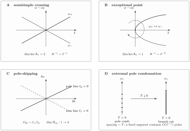
Four local fingerprints. A semisimple crossing keeps two vectors and gives a simple pole of the source-map inverse. An exceptional point has square-root sheets and a Jordan term. Pole-skipping is a two-variable indeterminacy caused by a jump in the ingoing horizon space. An extremal cut is the nonuniform limit of an infinite ladder.

Pole-skipping is a jump in the ingoing solution space

At a regular nonextremal horizon and generic $(\omega,k)$, future regularity selects one solution line. Suppose its boundary expansion is

$$\phi_{\mathrm{in}} = \alpha(\omega,k)B_- +\beta(\omega,k)B_+.$$

A common zero of $\alpha$ and $\beta$ in one chosen normalization can be an ordinary removable quotient. A candidate pole-skipping point is stronger: future regularity itself admits two independent solutions at $(\omega_*,k_*)$. Generic pole-skipping is confirmed only when the nearby ingoing line varies with approach direction and the UV map transports that variation nontrivially. There is then no unique pair $(\alpha,\beta)$ until one specifies how $(\omega,k)$ approaches the point.

For a generic transverse unfolding, the local response has the form

$$G_{\mathrm R}(\omega,k) = \mathcal C_* \frac{\delta\omega-v_z\delta k} {\delta\omega-v_p\delta k} +P_*+O(\delta),$$

where

$$\delta\omega=\omega-\omega_*, \qquad \delta k=k-k_*.$$

The pole line has slope $v_p$, while $v_z$ is the zero slope of the displayed nonlocal quotient. When $\mathcal C_*+P_*\ne0$, the zero of the full correlator instead has slope

$$\widetilde v_z = \frac{\mathcal C_*v_z+P_*v_p} {\mathcal C_*+P_*}.$$

Approaching along $\delta\omega=s\,\delta k$ still gives a value depending on $s$. A finite contact term changes the zero slope but not the underlying failure of horizon uniqueness; changing the boundary theory can also move the pole line.

This is not a Laurent double pole in $\omega$. It is a failure of a two-variable quotient to have a unique value at one point. Nor is it an exceptional point: the extra solution appears because the horizon condition loses rank, not because two global QNM eigenvectors necessarily form a Jordan chain.

The first scalar pole-skipping point comes from one horizon equation

Consider a minimally coupled scalar in an asymptotically AdS$_{d+2}$ black brane written in ingoing coordinates:

$$\dd s^2 = -r^2f(r)\dd v^2 +2\dd v\dd r +h(r)\dd\boldsymbol x_d^2.$$

Let $r=r_h$ be a nonextremal horizon with

$$f(r_h)=0, \qquad 4\pi T=r_h^2f'(r_h),$$

and set

$$\Phi = \ee^{-\ii\omega v+\ii kx}\phi(r).$$

The Klein–Gordon equation is

$$\begin{aligned} 0={}& \frac{\dd}{\dd r} \left[ h^{d/2} \left(r^2f\phi'-\ii\omega\phi\right) \right] \\ &- \ii\omega h^{d/2}\phi' -h^{d/2-1}(k^2+m^2h)\phi. \end{aligned}$$

Insert the future-regular Taylor series

$$\phi(r) = \phi_0+\phi_1(r-r_h)+\phi_2(r-r_h)^2+\cdots.$$

The horizon equation is

$$\begin{aligned} 0={}& -\left[ k^2+m^2h_h +\frac{\ii\omega d}{2}h_h' \right]\phi_0 \\ &+ (4\pi T-2\ii\omega)h_h\phi_1, \end{aligned}$$

where $h_h=h(r_h)$ and $h_h'=h'(r_h)$. Generically it fixes $\phi_1/\phi_0$, so regularity selects one line. At

$$\omega_1=-2\pi\ii T,$$

the coefficient of $\phi_1$ vanishes. The remaining coefficient vanishes too when

$$k_1^2 = -m^2h_h-d\pi T h_h'.$$

At $(\omega_1,k_1)$, both $\phi_0$ and $\phi_1$ are free. The two-dimensional local solution space is entirely future regular. Slightly away from the point, the leading horizon equation becomes

$$\begin{aligned} 0={}& -\left[ \frac{\ii d h_h'}{2}\delta\omega +2k_1\delta k \right]\phi_0 \\ &- 2\ii h_h\delta\omega\,\phi_1. \end{aligned}$$

Thus $\phi_1/\phi_0$ depends on the direction $\delta\omega/\delta k$. Radial transport carries that dependence to $\beta/\alpha$, producing the pole-skipping normal form. The horizon calculation locates the special point; the full geometry is still needed to determine the pole and zero slopes. This linear transverse unfolding assumes $k_1\ne0$ and a nondegenerate UV connection map. If $k_1=0$, momentum first enters through $(\delta k)^2$; the rank loss is anomalous in the linear $(\delta\omega,\delta k)$ chart and must be analyzed in $k^2$ or at higher order.

Higher Matsubara levels are finite rank tests

In ingoing coordinates, the two formal horizon exponents are

$$0, \qquad \frac{\ii\omega}{2\pi T}.$$

At

$$\omega_n=-2\pi\ii Tn, \qquad n=1,2,\ldots,$$

their difference is the positive integer $n$. A logarithm generically removes the second regular solution. Write the first $n$ Taylor equations as a finite system for $(\phi_0,\ldots,\phi_{n-1})$ and denote its coefficient matrix by $\mathcal M^{(n)}(\omega,k^2)$. The logarithmic obstruction vanishes on the horizon rank-loss, or apparent-singularity, locus

$$\det\mathcal M^{(n)}(\omega_n,k_n^2)=0.$$

The determinant condition locates the extra regular horizon solution, but it does not by itself guarantee the generic linear pole-skipping quotient. A simple transverse root, for example $\partial_k\det\mathcal M^{(n)}\ne0$, and a nondegenerate UV map are also needed. At $k_n=0$, or at a repeated root in $k^2$, varying $\delta\omega/\delta k$ need not sweep the two regular solutions; such an anomalous point requires a higher-order unfolding. The frequency $\omega=0$ likewise requires a separate analysis.

Static BTZ resolves the crossing in Gamma functions

Return to the nonresonant scalar quotient of the preceding page and set $r_-=0$, so $T_L=T_R=T$. With

$$\Delta=1+\nu=2h,$$

its nonlocal part is, up to a nonzero $(\omega,k)$-independent factor,

$$G_{\mathrm R}^{\mathrm{BTZ}} \sim \frac{ \Gamma(h-\ii q_L)\Gamma(h-\ii q_R) }{ \Gamma(1-h-\ii q_L) \Gamma(1-h-\ii q_R) },$$

where

$$q_L=\frac{\omega-k}{4\pi T}, \qquad q_R=\frac{\omega+k}{4\pi T}.$$

Assume noninteger $\nu$. On the plus-sign, positive-imaginary-momentum branch, the first intersection is

$$\omega_*=-2\pi\ii T, \qquad k_*=2\pi\ii T\nu,$$

the two Gamma arguments

$$x=h-\ii q_L, \qquad y=1-h-\ii q_R$$

both vanish. Since $\Gamma(x)\sim1/x$ and $1/\Gamma(y)\sim y$,

$$G_{\mathrm R}^{\mathrm{BTZ}} \sim \mathcal K_* \frac{y}{x} = \mathcal K_* \frac{\delta\omega+\delta k} {\delta\omega-\delta k},$$

with $\mathcal K_*\ne0$. The pole line $\delta\omega=\delta k$ and zero line $\delta\omega=-\delta k$ meet at a point where the hypergeometric horizon parameter is $c=0$. This is the exact boundary manifestation of the extra future-regular horizon solution. For compact BTZ, physical angular momentum is integer; the complex values of $k$ here belong to the analytic continuation used to define the two-variable Green function.

More generally, the static noninteger-$\nu$ intersections occur at

$$\begin{aligned} \omega_N&=-2\pi\ii TN, \\ k_{N,q} &= \pm2\pi\ii T(N-2q+\Delta), \end{aligned}$$

for $N=1,2,\ldots$ and $q=1,\ldots,N$. At integer $\nu$, logarithmic boundary renormalization changes the Gamma representation, and some rank-loss points can be anomalous. Use the logarithmic correlator itself rather than extrapolating the noninteger formula term by term.

The upper-half-plane energy-density point diagnoses chaos

For the energy-density correlator of a homogeneous static black-brane state with a classical two-derivative Einstein-gravity dual, and along a chosen spatial direction, the special upper-half-plane point is

$$\omega_\chi=\ii\lambda_L=2\pi\ii T, \qquad k_\chi=\ii\frac{\lambda_L}{v_B},$$

up to the sign of the spatial momentum. The same horizon Einstein equation controls the gravitational shock wave, which identifies the Lyapunov exponent $\lambda_L$ and butterfly velocity $v_B$.

This statement does not turn every pole-skipping point into a chaos diagnostic. The scalar points above lie at negative imaginary Matsubara frequencies, their momenta depend on the scalar mass and horizon geometry, and they are generically unrelated to $v_B$. Conserved-current and stress-tensor channels also possess lower-half-plane towers that constrain collective-mode and transport dispersion, but are not universal scrambling data.

Extremality changes the endpoint class

For a rotating and charged perturbation, the frequency measured by the future horizon generator is

$$\widehat\omega = \omega-m_\varphi\Omega_H-q_\Phi\Phi_H.$$

Here $m_\varphi$ is the azimuthal number, $q_\Phi$ is the field charge, and the electrostatic potential is defined relative to the boundary gauge. $\widehat\omega$ is the natural horizon-frame variable. A limiting calculation must then declare whether it holds $\widehat\omega$ fixed or instead resolves a scaled throat variable such as $\widehat\omega/T$.

At a nonextremal horizon, a Schwarzschild-like radial function $F(r)$ has a simple zero. At an extremal horizon it has a double zero:

$$\begin{array}{c|c|c} &F(r)&r_*'=F^{-1} \\ \hline T>0 &4\pi T(r-r_h)+\cdots &\displaystyle r_*\sim\frac{\log(r-r_h)}{4\pi T} \\ T=0 &\alpha(r-r_h)^2+\cdots &\displaystyle r_*\sim-\frac1{\alpha(r-r_h)} \end{array}$$

For a Schwarzschild-time ansatz $\Phi=\ee^{-\ii\omega t+\ii m_\varphi\varphi}R(r)$, the nonextremal ingoing radial factor is consequently a Frobenius power, whereas the generic extremal factor is essential:

$$\begin{aligned} R_{\mathrm{in}}^{T>0} &\sim (r-r_h)^{-\ii\widehat\omega/(4\pi T)}, \\ R_{\mathrm{in}}^{T=0} &\sim \exp\!\left[ \frac{\ii\widehat\omega}{\alpha(r-r_h)} \right]. \end{aligned}$$

In ingoing Eddington–Finkelstein coordinates the same future solution is regular; the singular factors above are carried by the change from $t$ to the ingoing time. Their different dependence on $r-r_h$ is what changes the separated radial endpoint from regular singular to irregular.

In the exact extremal radial equation the horizon is therefore generically irregular. Taking $T\to0$ coefficient by coefficient in a nonextremal Frobenius series cannot reproduce this endpoint. A branch cut is not automatic for every field and every observable, but when a nondegenerate throat channel survives the connection to infinity, the change of endpoint class explains why an infinite thermal pole family can have a nonmeromorphic limit.

Rotating BTZ turns a thermal ladder into a branch cut

The preceding page gives an exact laboratory. For a noninteger $\nu=2h-1$, remove the contact term and write the rotating-BTZ correlator as

$$G_{\mathrm R,\mathrm{nloc}} = \mathcal C_{\mathrm{BTZ}} D^\nu\mathcal R_L\mathcal R_R,$$

where

$$\begin{aligned} \mathcal C_{\mathrm{BTZ}} &= 2\nu\mathcal N_\Phi \frac{\Gamma(-\nu)}{\Gamma(\nu)}, \\ D&=4\pi^2T_LT_R, \\ \mathcal R_L &= \frac{\Gamma(h-\ii q_L)} {\Gamma(1-h-\ii q_L)}, \\ \mathcal R_R &= \frac{\Gamma(h-\ii q_R)} {\Gamma(1-h-\ii q_R)}. \end{aligned}$$

Take the extremal limit $T_L\to0$ with $T_R$ and $p=\omega-k$ fixed. Since $\Omega_H\to1$ and $m_\varphi=k$ for the BTZ angular mode, $p$ is precisely the neutral horizon-frame threshold variable. The Gamma-ratio asymptotic formula gives

$$\frac{\Gamma(h-\ii q_L)} {\Gamma(1-h-\ii q_L)} \sim (-\ii q_L)^\nu, \qquad q_L=\frac{p}{4\pi T_L},$$

and hence

$$D^\nu\mathcal R_L \longrightarrow \left[-\ii\pi T_R(\omega-k)\right]^\nu.$$

The exact fixed-frequency limit of the nonlocal part is therefore

$$\begin{aligned} G_{\mathrm R,\mathrm{nloc}}^{\mathrm{ext}} ={}& \mathcal C_{\mathrm{BTZ}} \left[-\ii\pi T_R(\omega-k)\right]^\nu \\ &\times \frac{ \Gamma\!\left( h-\dfrac{\ii(\omega+k)}{4\pi T_R} \right) }{ \Gamma\!\left( 1-h-\dfrac{\ii(\omega+k)}{4\pi T_R} \right) }. \end{aligned}$$

For noninteger $\nu$, the first factor has a branch point at $\omega=k$. Choosing the retarded function analytic in the upper half-plane places a convenient cut vertically downward from that point. The cut direction is conventional; the branch point and its nontrivial monodromy are not. Once a cut is chosen, local contact terms are analytic and cannot cancel its jump.

At every $T_L>0$, the same factor is meromorphic. Its left-moving poles and zeros are

$$\begin{aligned} \omega_n^{\mathrm{pole}} &= k-4\pi\ii T_L(n+h), \\ \omega_n^{\mathrm{zero}} &= k-4\pi\ii T_L(n+1-h), \end{aligned}$$

with $n=0,1,2,\ldots$, apart from accidental cancellations. To reach a fixed point $\omega=k-\ii y$ on the limiting cut, one needs

$$n\sim\frac{y}{4\pi T_L}\longrightarrow\infty.$$

This is the essential nonuniformity. No finite pair of poles collides to create the cut. At fixed $n$, every left-moving pole merely approaches the endpoint $\omega=k$; at fixed $\omega-k$, an unbounded number of poles and zeros fills the intervening segment.

If the remaining right-moving factor is regular and nonzero at $\omega=k$, the cut contribution to the late-time response scales as

$$G_{\mathrm R}^{\mathrm{cut}}(t) \propto \ee^{-\ii kt}t^{-\nu-1}.$$

For positive integer $\nu$, one must first renormalize the full correlator. If the remaining right-moving factor is regular and nonzero, the generic nonlocal limit contains a power times $\log[-\ii(\omega-k)]$ and gives the same algebraic exponent, although special coefficients can cancel the logarithm. At an exceptional momentum where that factor is singular—most notably the $\nu=1$ extremal pole-skipping locus discussed below—the tail must be analyzed from the complete quotient. The BF-bound case $\nu=0$ and imaginary $\nu$ require their own limiting analyses.

Two limits that answer different questions

Holding $q_L=(\omega-k)/(4\pi T_L)$ fixed zooms into a thermal throat window whose width shrinks with $T_L$. Holding $\omega-k$ fixed probes the outer frequency plane and produces the branch function above. Interchanging these limits discards either the resolved pole comb or its limiting cut.

Thermal AdS₂ is a canonical throat model

The same mechanism appears without relying on the special functions of BTZ. For a neutral mode in a thermal AdS$_2$ throat, absorb transverse momentum and other separation data into $m_{\mathrm{eff}}$ and define

$$\delta_{\mathrm{IR}} = \frac12+\nu_{\mathrm{IR}}, \qquad \nu_{\mathrm{IR}} = \sqrt{ \frac14+m_{\mathrm{eff}}^2L_2^2 }.$$

For real $\nu_{\mathrm{IR}}$ with $2\nu_{\mathrm{IR}}\notin\mathbb Z$, one convenient normalization of the retarded throat function is

$$\begin{aligned} \mathcal G_T^{\mathrm R}(\widehat\omega) ={}& C_{\mathrm{IR}}(4\pi T)^{2\nu_{\mathrm{IR}}} \\ &\times \frac{ \Gamma\!\left( \delta_{\mathrm{IR}} -\dfrac{\ii\widehat\omega}{2\pi T} \right) }{ \Gamma\!\left( 1-\delta_{\mathrm{IR}} -\dfrac{\ii\widehat\omega}{2\pi T} \right) }, \end{aligned}$$

where

$$C_{\mathrm{IR}} = \frac{ \Gamma(-2\nu_{\mathrm{IR}}) \Gamma(\delta_{\mathrm{IR}}) }{ \Gamma(2\nu_{\mathrm{IR}}) \Gamma(1-\delta_{\mathrm{IR}}) }.$$

Its thermal poles and zeros form interlaced ladders,

$$\begin{aligned} \widehat\omega_n^{\mathrm{pole}} &= -2\pi\ii T(n+\delta_{\mathrm{IR}}), \\ \widehat\omega_n^{\mathrm{zero}} &= -2\pi\ii T(n+1-\delta_{\mathrm{IR}}). \end{aligned}$$

At fixed $\widehat\omega$, Stirling’s formula yields

$$\mathcal G_T^{\mathrm R}(\widehat\omega) \longrightarrow C_{\mathrm{IR}}2^{2\nu_{\mathrm{IR}}} (-\ii\widehat\omega)^{2\nu_{\mathrm{IR}}}.$$

Thus the finite-temperature pole spacing resolves the exact extremal branch point at the horizon-frame threshold $\widehat\omega=0$.

The throat function is not yet the full boundary correlator. In the matched low-$T$, low-$\widehat\omega$ regime, with both small relative to the UV scale, transport through the outer region gives the Möbius connection formula

$$G_{\mathrm R} = \mathcal K \frac{ b_+(\omega,k) +b_-(\omega,k)\mathcal G_T^{\mathrm R} }{ a_+(\omega,k) +a_-(\omega,k)\mathcal G_T^{\mathrm R} } +P_{\mathrm{loc}},$$

where $a_\pm$ and $b_\pm$ are analytic outer connection coefficients. The poles of $\mathcal G_T^{\mathrm R}$ are therefore not automatically the exact QNMs of the full geometry; those solve the zero of the displayed denominator. The Möbius map depends nontrivially on the throat data when

$$a_+b_- - a_-b_+\ne0$$

at the threshold. Under that nondegeneracy condition, the full response inherits the IR branch point and its near-extremal QNMs accumulate toward the cut.

This picture has several concrete realizations. In RN–AdS$_5$, the low-$T$ Heun equation undergoes a confluent limit as two regular singularities coalesce, and the controlled double scaling $\omega,T\to0$ at fixed $\omega/T$ analytically resolves the emergence of the zero-temperature cut. In extremal Kerr, the horizon branch point is at the superradiant threshold $\omega=m_\varphi\Omega_H$, where a family of near-extremal modes accumulates. An asymptotically flat spacetime may also have a separate branch point at $\omega=0$ from its long-range potential at infinity; that outer-endpoint cut must not be attributed to the extremal horizon.

In a one-temperature or horizon-frame scaling, fixed-$n$ pole-skipping points can collapse toward $\widehat\omega=0$, but that observation alone does not define pole-skipping in the exact extremal equation. Rotating BTZ makes the coordinate caveat explicit: as $T_L\to0$ with $T_R$ finite, nonextremal points can approach finite boundary frequencies on $\omega=k$, even though their left-moving horizon-frame offset vanishes. The exact-extremal horizon recursion must be rebuilt. For a minimally coupled BTZ scalar, generic noninteger $\nu$ and positive integers $\nu>1$ do not yield slope-type extremal pole-skipping; the special $\nu=1$ case survives at

$$\omega=k=-2\pi\ii T_R(n+1), \qquad n=0,1,2,\ldots.$$

Pole condensation and pole-skipping therefore remain distinct even when their finite-temperature plots approach the same frequency.

A diagnostic workflow that survives numerical noise

Use the following order rather than classifying a dense scatter plot by eye:

1. Freeze the problem. Record the perturbation sector, gauge quotient, boundary condition, parameter sheet, and whether each endpoint selects one solution line.

2. Normalize the analytic object. Use regular, unit-leading endpoint bases. Ignore invertible holomorphic changes; remove a vanishing or singular factor only when an independent derivation identifies it as a basis artifact.

3. Count zeros topologically. If $D$ is holomorphic inside $\Gamma$ and nonzero on the contour, evaluate

   $$m = \frac1{2\pi\ii} \oint_\Gamma \frac{\partial_\omega D}{D}\dd\omega.$$

   This counts its enclosed zeros with multiplicity. For meromorphic $D$, the same integral counts zeros minus poles. Shrink and refine $\Gamma$ to distinguish a multiple zero from an unresolved cluster.

4. Measure the nullspace. Compute both left and right null vectors, monitor singular-value convergence with precision, and evaluate the crossing matrix $K$. Solve the generalized-vector equation before declaring an exceptional point.

5. Audit projections. Reconstruct the matrix Laurent coefficients. A scalar observable may cancel the highest principal part or the entire mode.

6. Test pole-skipping in two variables. Approach the candidate along several slopes in $(\omega,k)$ and verify the horizon-rank jump. A common numerator and denominator zero in one chart is not enough.

7. Test a proposed cut as a family. Decrease $T$, count poles in a fixed frequency segment, verify that the count grows like $T^{-1}$, and compare with an independently computed discontinuity or limiting connection formula.

8. Check the time domain. A semisimple crossing gives a sum of exponentials, an EP can give $t\ee^{-\ii\omega_*t}$, and a cut gives a continuum integral with an algebraic tail. These signatures corroborate the analytic test; they do not replace it.

The essential fingerprints are compactly summarized here:

Phenomenon	Local object	Decisive test	Generic response
Semisimple crossing	Global source map	$m_{\mathrm{alg}}=m_{\mathrm{geo}}=2$	$\mathsf A^{-1}$ has a simple pole and rank-two residue before projection
Order-two exceptional point	Global source map	$m_{\mathrm{alg}}=2$, $m_{\mathrm{geo}}=1$	$\mathsf A^{-1}$ has a double pole; a projection can show $t\ee^{-\ii\omega_*t}$
Pole-skipping	Horizon regularity map in $(\omega,k)$	Ingoing dimension jumps and the unfolding is transverse	Direction-dependent pole–zero quotient
Extremal branch point	Limit of a meromorphic family	Infinite nonuniform condensation and nonzero discontinuity	Cut integral and algebraic tail

Common pitfalls

Equating a double determinant zero with an exceptional point. The semisimple and defective normal forms can have the same zero multiplicity. Test the kernel dimension, crossing matrix, and Laurent order.

Calling every square root an eigenvector defect. Eliminating an angular accessory parameter or choosing a ramified control coordinate can create square-root branches. Restore the full analytic map and use a local uniformizer.

Diagnosing pole-skipping from a canceled quotient. A numerator and denominator can share a removable factor while the horizon still selects a unique solution. Verify a second future-regular solution and slope dependence near the point.

Calling a finite pole cluster a branch cut. Any finite collection is still meromorphic. Demonstrate growth of the pole count in a controlled limit and identify the limiting discontinuity.

Taking extremality at fixed overtone number. Fixed-$n$ poles only reveal the branch-point endpoint. The cut is built from $n\sim T^{-1}$, while the exact extremal horizon requires a new irregular-endpoint analysis.

Exercises

1. Equal determinant order, unequal resolvent order

At the collision point, compute the determinant order, kernel dimension, and inverse pole order of $\mathsf A_{\mathrm{ss}}$ and $\mathsf A_{\mathrm{EP}}$. Explain why only one model can produce a term $t\ee^{-\ii\omega_0t}$.

Solution

At $\lambda=0$, both determinants equal $\delta^2$, so both have algebraic multiplicity two. For the semisimple model, $\mathsf A_{\mathrm{ss}}=\delta\mathsf I_2$, hence the kernel at $\delta=0$ has dimension two and the inverse is $\delta^{-1}\mathsf I_2$. Its pole is simple.

For the exceptional-point model,

$$\mathsf A_{\mathrm{EP}}(0,0) = \begin{pmatrix}0&-1\\0&0\end{pmatrix},$$

whose kernel is spanned by $(1,0)^{\mathsf T}$. Its inverse contains $\delta^{-2}$, so a projection that sees this entry has a double pole. The inverse transform of $\ee^{-\ii\omega t}/(\omega-\omega_0)^2$ is proportional to $t\ee^{-\ii\omega_0t}$; a simple pole gives only an exponential.

2. Crossing-matrix test

Evaluate $K$ for the two normal forms at $\lambda=0$. For the exceptional-point model, construct one right generalized vector $v_1$.

Solution

For the semisimple model, choose $Z_L=Z_R=\mathsf I_2$. Since $\partial_\omega\mathsf A_{\mathrm{ss}}=\mathsf I_2$, one obtains $K=\mathsf I_2$, so the double root is semisimple.

For the exceptional-point model, take

$$v_0=\begin{pmatrix}1\\0\end{pmatrix}, \qquad w_0^{\mathsf T}=\begin{pmatrix}0&1\end{pmatrix}.$$

Then $K=w_0^{\mathsf T}v_0=0$. The chain equation is $\mathsf A_*v_1+v_0=0$, and one choice is

$$v_1=\begin{pmatrix}0\\1\end{pmatrix}.$$

The vanishing crossing matrix and solvable chain equation diagnose the defect.

3. First pole-skipping momentum of an AdS black brane

For the planar Schwarzschild–AdS$_{d+2}$ metric in the ingoing chart above, take

$$h(r)=r^2, \qquad f(r)=1-\left(\frac{r_h}{r}\right)^{d+1}.$$

For a massless scalar, express $T$ and $k_1^2$ in terms of $r_h$.

Solution

Since $f'(r_h)=(d+1)/r_h$,

$$T=\frac{(d+1)r_h}{4\pi}.$$

Also $h_h=r_h^2$ and $h_h'=2r_h$. The first horizon condition gives

$$\begin{aligned} k_1^2 &=-d\pi T(2r_h) \\ &=-\frac{d(d+1)}2r_h^2. \end{aligned}$$

The momentum is imaginary on either square-root branch, as expected for this lower-half-plane pole-skipping point.

4. Resolve the first BTZ pole-skipping point

At

$$(\omega_*,k_*) = (-2\pi\ii T,2\pi\ii T\nu),$$

show directly that

$$x=h-\ii q_L = -\frac{\ii(\delta\omega-\delta k)}{4\pi T},$$

and

$$y=1-h-\ii q_R = -\frac{\ii(\delta\omega+\delta k)}{4\pi T}.$$

Deduce the slope-dependent quotient.

Solution

Substitution of $\omega_*$ and $k_*$ gives $x_*=y_*=0$. Their dependence on $\omega$ and $k$ is affine, so the displayed variations are exact. Near zero, $\Gamma(x)\sim x^{-1}$ and $1/\Gamma(y)\sim y$. All other Gamma factors are finite and nonzero for generic noninteger $\nu$. Therefore

$$G_{\mathrm R} \sim \mathcal K_* \frac{\delta\omega+\delta k} {\delta\omega-\delta k} +P_*.$$

Along $\delta\omega=s\,\delta k$, the nonlocal quotient approaches $\mathcal K_*(s+1)/(s-1)$, which is not a unique value at the intersection.

5. From the BTZ pole comb to the late-time tail

Use the large-argument Gamma-ratio formula to derive the extremal BTZ branch factor. Then show that a local factor $[-\ii(\omega-k)]^\nu$, with noninteger $\nu>-1$, contributes a late-time power $\ee^{-\ii kt}t^{-\nu-1}$ when the remaining factors are regular.

Solution

The asymptotic relation

$$\frac{\Gamma(z+a)}{\Gamma(z+b)} \sim z^{a-b}$$

with $z=-\ii q_L$, $a=h$, and $b=1-h$ gives $\mathcal R_L\sim(-\ii q_L)^\nu$. Since $D=4\pi^2T_LT_R$,

$$D^\nu\mathcal R_L \longrightarrow [-\ii\pi T_R(\omega-k)]^\nu.$$

On the downward cut write $\omega-k=-\ii y$, $y>0$. The discontinuity of the fractional power is a nonzero constant times $y^\nu$. The cut integral then contains

$$\ee^{-\ii kt} \int_0^\infty \ee^{-yt}y^\nu\dd y = \Gamma(\nu+1) \ee^{-\ii kt}t^{-\nu-1}.$$

Analytic prefactors change the coefficient but not this leading exponent unless they vanish at the branch point.

6. Why fixed overtone number misses the cut

For the BTZ left-moving ladder, estimate how many poles lie between $\omega=k$ and $\omega=k-\ii Y$ at small $T_L$. Explain why following the first ten overtones cannot establish the extremal cut.

Solution

The imaginary spacing is $4\pi T_L$, so the number in a fixed segment is

$$N(Y,T_L) = \frac{Y}{4\pi T_L}+O(1).$$

It diverges as $T_L^{-1}$. Every fixed overtone instead approaches $\omega=k$, revealing only the endpoint. A fixed list of ten modes never samples points a finite distance down the limiting cut; one must increase the overtone range proportionally to $T_L^{-1}$ and compare with the limiting branch discontinuity.

References

• T. Kato, Perturbation Theory for Linear Operators, 2nd ed. (Springer).
• J. M. Schumacher, “Keldysh’s theorem revisited,” Linear Algebra and its Applications 730 (2026) 358–386 (journal).
• O. Gannot, “A global definition of quasinormal modes for Kerr–AdS black holes,” Annales de l’Institut Fourier 68 (2018) 1125–1167 (journal).
• R. da C. Cavalcante, M. Richartz, and B. Carneiro da Cunha, “Exceptional Point and Hysteresis in Perturbations of Kerr Black Holes,” Physical Review Letters 133 (2024) 261401 (journal).
• H. Motohashi, “Resonant Excitation of Quasinormal Modes of Black Holes,” Physical Review Letters 134 (2025) 141401 (journal).
• M. Blake, R. A. Davison, and D. Vegh, “Horizon constraints on holographic Green’s functions,” Journal of High Energy Physics 2020(1) 77 (journal).
• M. Blake, R. A. Davison, S. Grozdanov, and H. Liu, “Many-body chaos and energy dynamics in holography,” Journal of High Energy Physics 2018(10) 35 (journal).
• M. Natsuume and T. Okamura, “Pole-skipping and zero temperature,” Physical Review D 103 (2021) 066017 (journal).
• T. Faulkner, H. Liu, J. McGreevy, and D. Vegh, “Emergent quantum criticality, Fermi surfaces, and AdS$_2$,” Physical Review D 83 (2011) 125002 (journal).
• P. Arnaudo and B. Withers, “Exact low-temperature Green’s functions in AdS/CFT: From the Heun equation to the confluent Heun equation,” Physical Review D 111 (2025) L121903 (journal, arXiv:2412.01923).
• M. Casals, S. E. Gralla, and P. Zimmerman, “Horizon instability of extremal Kerr black holes: Nonaxisymmetric modes and enhanced growth rate,” Physical Review D 94 (2016) 064003 (journal).
• M. Casals and L. F. Longo Micchi, “Spectroscopy of extremal and near-extremal Kerr black holes,” Physical Review D 99 (2019) 084047 (journal).