Confluence and Singular Limits

Confluence turns several singular points into one, but geometric collision is only the visible part of the process. The limiting equation depends on how coordinates, residues, parameters, branches, and solution bases scale. Two colliding Fuchsian poles with bounded residues remain Fuchsian; an irregular limit requires a polar moment to survive.

The same care is needed for analytic data. Initial-value solutions can converge on a common outer domain while Frobenius eigenbases diverge, local monodromy matrices oscillate, and their connection matrices require singular right normalizations. A Stokes matrix is therefore a limit of normalized connection data in a declared parameter sector, not generically the limit of one raw monodromy matrix.

Confluence is a scaling statement

“Let two singularities merge” does not define a limit. State the coordinate map and its inverse, which variable is fixed, how the residues scale, the approach direction of the parameter, the branches, the basis renormalizations, and the domain on which convergence is claimed.

The algebra of a two-pole collision

Center the collision at $x=a$ and set $u=x-a$. Consider

$$\frac{\dd Y}{\dd u} = \left[ \frac{A_+(\varepsilon)}{u-\varepsilon} +\frac{A_-(\varepsilon)}{u+\varepsilon} +R_\varepsilon(u) \right]Y,$$

where $R_\varepsilon$ is holomorphic near the cluster. Assume also that $R_\varepsilon\to R_0$ locally uniformly there; it then contributes only a holomorphic term to the outer limit. The exact identity

$$\frac{A_+}{u-\varepsilon} +\frac{A_-}{u+\varepsilon} = \frac{ u(A_++A_-) +\varepsilon(A_+-A_-) }{ u^2-\varepsilon^2 }$$

separates the zeroth and first polar moments.

Bounded residues give a regular limit

Suppose $A_\pm(\varepsilon)$ have finite limits. For fixed $u\neq0$,

$$\frac{A_+}{u-\varepsilon} +\frac{A_-}{u+\varepsilon} \longrightarrow \frac{A_+(0)+A_-(0)}{u}.$$

The two simple poles have merged into one simple pole. Collision by itself has not created irregularity.

Opposite residue blow-up gives a double pole

Now scale the residues as

$$\begin{aligned} A_+(\varepsilon) &= \frac{B_2}{2\varepsilon} +\frac{B_1}{2} +O(\varepsilon),\\ A_-(\varepsilon) &= -\frac{B_2}{2\varepsilon} +\frac{B_1}{2} +O(\varepsilon). \end{aligned}$$

On compact subsets with $u\neq0$,

$$\frac{A_+}{u-\varepsilon} +\frac{A_-}{u+\varepsilon} \longrightarrow \frac{B_2}{u^2} +\frac{B_1}{u}.$$

The residues diverge oppositely, so their sum stays finite while their first moment survives as $B_2$. This is the elementary mechanism behind a Poincaré-rank-one irregular confluence.

If $B_2$ is semisimple with distinct eigenvalues $\lambda_j$, diagonalize it by a constant basis change. The first formal reduction gives

$$\widehat\Phi(u) = \widehat H(u) \exp\left(-\frac{B_2^{\mathrm d}}{u}\right) u^\Lambda,$$

where, in this nonresonant leading situation, $\Lambda$ is the diagonal part of $B_1$ in the $B_2$-eigenbasis. The exponential factors are

$$q_j(u)=-\frac{\lambda_j}{u}.$$

The displayed double pole is not by itself an invariant rank calculation:

• scalar $B_2$ gives a common $GL_n$ exponential but no projective exponential separation;
• nilpotent $B_2$ may be removable or may require shearing before the slopes are visible;
• coalescing eigenvalues of $B_2$ define a separate parameter stratum on which the formal type must be recomputed.

For a loop enclosing the full two-pole cluster, Abel’s determinant identity provides a useful check:

$$\det M_{\mathrm{cluster}} \longrightarrow \exp\left( 2\pi\ii\,\operatorname{tr}B_1 \right).$$

This agrees with the determinant of the limiting formal monodromy because all Stokes factors are unipotent.

Outer, inner, and parameter domains

A singular perturbation has more than one meaningful limit.

Domain	Variable held fixed	What it resolves
Outer	$u=x-a$	The merged irregular equation away from the shrinking cluster
Inner	$s=u/\varepsilon$	The two distinct points $s=\pm1$ and their local interaction
Parameter sector	$\arg\varepsilon$ in a fixed interval	Branches, sector labels, dominance order, and normalized analytic limits

On the inner scale,

$$\frac{\dd Y}{\dd s} = \left[ \frac{A_+(\varepsilon)}{s-1} +\frac{A_-(\varepsilon)}{s+1} +\varepsilon R_\varepsilon(\varepsilon s) \right]Y.$$

For the irregular residue scaling above, this is a large-parameter problem because $A_\pm=O(\varepsilon^{-1})$. It is not obtained by simply inserting $u=0$ into the outer limiting equation.

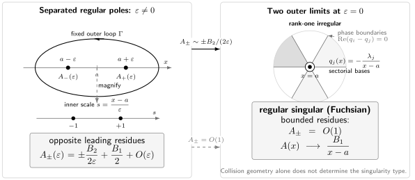
Outer and inner views of a two-pole collision. Geometric coalescence produces an irregular point only when the residues scale oppositely as $\pm B_2/(2\varepsilon)$; bounded residues produce a regular singular limit. A fixed outer loop probes the full limiting analytic monodromy, while $s=(x-a)/\varepsilon$ keeps the two perturbed poles apart.

There is nevertheless a robust outer convergence statement. Let $D$ be a common simply connected domain avoiding the moving cluster, choose a fixed base point $u_*\in D$, and suppose

$$A_\varepsilon \longrightarrow A_0$$

uniformly on compact subsets of $D$. The normalized fundamental matrices

$$\Phi_\varepsilon(u_*)=I$$

satisfy a Volterra integral equation. Standard successive approximation then gives

$$\Phi_\varepsilon \longrightarrow \Phi_0$$

locally uniformly on $D$.

This theorem says nothing about shrinking Frobenius disks, the inner scale, or canonical eigenbases whose exponents grow like $\varepsilon^{-1}$. For branch-dependent canonical bases, however, one must additionally restrict $\varepsilon$ to a parameter sector: a spiraling approach can continually change logarithm branches and sector labels.

From connection matrices to Stokes matrices

Let $F_-$ and $F_+$ be canonical bases associated with the two perturbed singularities, analytically continued to a common domain, and write

$$F_+=F_-C_{-+}.$$

These raw bases often have no limit. Choose right normalizers $K_\pm(\varepsilon)$ and a fixed parameter ray such that

$$\begin{aligned} F_-K_-&\longrightarrow\Phi_k,\\ F_+K_+&\longrightarrow\Phi_{k+1}, \end{aligned}$$

where $\Phi_k$ and $\Phi_{k+1}$ are adjacent normalized sectorial bases of the irregular limiting equation. Then

$$F_+K_+ = F_-K_- \left( K_-^{-1}C_{-+}K_+ \right),$$

so the book’s right-action convention gives

$$S_k = \lim_{\varepsilon\to0} K_-^{-1}C_{-+}K_+, \qquad \Phi_{k+1}=\Phi_kS_k.$$

This formula is basis covariant and exposes every normalization used in the limit. Different parameter sectors can select different adjacent sectorial bases and therefore different Stokes factors.

Three limits must remain distinct:

Perturbed datum	Possible normalized limit
One connection matrix between selected local bases	One Stokes factor $S_k$
Monodromy of a fixed loop enclosing the cluster	Full analytic monodromy $M_\gamma$
One raw local monodromy matrix	Generically neither of the above

With the crossing convention of sectorial normalization,

$$M_\gamma = M_{\mathrm f} S_{m-1}^{-1}\cdots S_0^{-1}.$$

Thus a cluster loop cannot generally isolate one jump. In generic perturbations, even an individual monodromy operator need not converge to a Stokes operator; special normalized products or connection data are required.

Gauss becomes Kummer

The classical hypergeometric confluence provides an exact scalar benchmark. Use $B$ for the large parameter and start from

$$x(1-x)y_{xx} +\left[ c-(a+B+1)x \right]y_x -aB\,y=0.$$

Set

$$x=\frac zB, \qquad y(x)=u_B(z).$$

Because

$$y_x=B u_B', \qquad y_{xx}=B^2u_B'',$$

division by $B$ gives the exact scaled equation

$$\begin{aligned} z\left(1-\frac zB\right)u_B'' &+ \left[ c-z-\frac{(a+1)z}{B} \right]u_B'\\ &-a\,u_B=0. \end{aligned}$$

On compact subsets of the finite $z$-plane,

$$z u''+(c-z)u'-a u=0,$$

which is Kummer’s equation. At finite $B$, the points $z=0,B,\infty$ are regular singular. In $t=1/z$, the points $t=1/B$ and $t=0$ merge; the limiting point $z=\infty$ has Poincaré rank one.

Both Frobenius branches need normalization

Assume $c\notin\mathbb Z$ and fix compatible branches of $\operatorname{Log}B$ and $\operatorname{Log}(z/B)$. A Frobenius pair at $z=0$ is

$$\begin{aligned} u_{1,B}(z) &= {}_2F_1 \left( a,B;c;\frac zB \right),\\ u_{2,B}(z) &= B^{1-c} \left(\frac zB\right)^{1-c} {}_2F_1 \left( \begin{matrix} a+1-c,\ B+1-c\\ 2-c \end{matrix} ;\frac zB \right). \end{aligned}$$

For each fixed series index,

$$\frac{(B)_n}{B^n}\longrightarrow1,$$

and the resulting series limits are locally uniform in $z$. Hence

$$\begin{aligned} u_{1,B}(z) &\longrightarrow {}_1F_1(a;c;z),\\ u_{2,B}(z) &\longrightarrow z^{1-c} {}_1F_1(a+1-c;2-c;z). \end{aligned}$$

The factor $B^{1-c}$ is indispensable: without it, the second Frobenius normalization contains a factor $B^{c-1}$, which generally has no finite nonzero limit. When $c\in\mathbb Z$, the two Frobenius exponents are resonant and the basis must be recombined before taking the limit.

The basic power-to-exponential mechanism is

$$\left( 1-\frac zB \right)^{c-a-B} \longrightarrow \ee^z$$

on a domain and parameter sector where the logarithm is fixed.

Kummer’s limiting formal and Stokes data

For

$$z u''+(c-z)u'-a u=0,$$

the scalar coefficients are

$$p(z)=\frac cz-1, \qquad q(z)=-\frac az.$$

The Liouville substitution

$$u=\ee^{z/2}z^{-c/2}\psi$$

gives

$$\psi'' +\left[ -\frac14 +\frac{c-2a}{2z} +\frac{c(2-c)}{4z^2} \right]\psi=0.$$

One convenient ordered formal basis at infinity is

$$\begin{aligned} \widehat u_{\mathrm e}(z) &= \ee^z z^{a-c} {}_2F_0 \left( c-a,1-a;\,;\,z^{-1} \right),\\ \widehat u_{\mathrm a}(z) &= -z^{-a} {}_2F_0 \left( a,a+1-c;\,;\,-z^{-1} \right). \end{aligned}$$

The labels refer to the exponential and algebraic branches; the minus sign fixes the normalization used below. With $t=1/z$, a positive $t$-loop makes $z$ turn clockwise. The resulting formal monodromy is

$$M_{\mathrm f} = \operatorname{diag} \left( \ee^{2\pi\ii(c-a)}, \ee^{2\pi\ii a} \right).$$

The exponential difference is $q_{\mathrm e}-q_{\mathrm a}=z$. Therefore:

• equal magnitude occurs on $\operatorname{Re}z=0$;
• $\exp(q_{\mathrm e}-q_{\mathrm a})$ is maximally decaying at $\arg z=\pi$;
• the reverse ordered difference is maximally decaying at $\arg z=0$.

Expert checkpoint: exact Kummer multipliers

On the universal cover, let

$$\Sigma_k = \left\{ -\frac{\pi}{2} < \arg z-k\pi < \frac{3\pi}{2} \right\},$$

and let the canonical bases asymptotic to the ordered formal basis above satisfy $\Phi_{k+1}=\Phi_kS_k$. For generic $a,c$, one compatible normalization gives

$$S_0 = I+ \frac{ 2\pi\ii\,\ee^{\ii\pi(c-2a)} }{ \Gamma(a)\Gamma(a+1-c) } E_{12},$$

and

$$S_{-1} = I+ \frac{ 2\pi\ii }{ \Gamma(1-a)\Gamma(c-a) } E_{21}.$$

Reciprocal gamma functions continue the multipliers through many degenerate parameter values, but a coalescing canonical basis still has to be treated separately. In the Gauss family, normalized connection matrices approach $S_0$ or $S_{-1}$ along different large-$B$ parameter directions. The parameter ray is therefore part of the theorem, not a cosmetic choice.

A triangular unfolding with visible signs

The preceding page’s Borel–Laplace model has a particularly transparent Fuchsian unfolding:

$$\frac{\dd Y}{\dd x} = \frac{1}{x^2-\varepsilon^2} \begin{pmatrix} -1&x\\ 0&0 \end{pmatrix}Y.$$

For $\varepsilon\neq0$, the two poles are regular singular, with residues

$$R_+ = \begin{pmatrix} -\dfrac{1}{2\varepsilon}&\dfrac12\\ 0&0 \end{pmatrix}, \qquad R_- = \begin{pmatrix} \dfrac{1}{2\varepsilon}&\dfrac12\\ 0&0 \end{pmatrix}.$$

The nontrivial local monodromy eigenvalues are

$$\ee^{-\pi\ii/\varepsilon} \quad\text{and}\quad \ee^{\pi\ii/\varepsilon},$$

so the individual monodromy matrices generally have no limit. The homogeneous first component is

$$g_\varepsilon(x) = \left( \frac{x-\varepsilon}{x+\varepsilon} \right)^{-1/(2\varepsilon)}.$$

On compact subsets away from $x=0$, with continuously chosen logarithms,

$$\begin{aligned} \log g_\varepsilon &= -\frac{1}{2\varepsilon} \left[ \operatorname{Log}\left(1-\frac{\varepsilon}{x}\right) -\operatorname{Log}\left(1+\frac{\varepsilon}{x}\right) \right]\\ &\longrightarrow\frac1x. \end{aligned}$$

Thus $g_\varepsilon\to\ee^{1/x}$, and the coefficient matrix tends to

$$\begin{pmatrix} -x^{-2}&x^{-1}\\ 0&0 \end{pmatrix},$$

exactly the irregular triangular system already summed on the sectorial page.

To compute the cluster monodromy without taking a delicate product of local eigenbases, set $t=1/x$. The system becomes

$$\frac{\dd Y}{\dd t} = \begin{pmatrix} \dfrac{1}{1-\varepsilon^2t^2} & -\dfrac{1}{t(1-\varepsilon^2t^2)} \\ 0&0 \end{pmatrix}Y.$$

Write the upper entry of the second column as $h_\varepsilon=g_\varepsilon v_\varepsilon$, now regarding $g_\varepsilon$ as a function of $t$. Then

$$v_\varepsilon' = -\frac{1}{ t(1-\varepsilon^2t^2)g_\varepsilon(t) },$$

and, since $g_\varepsilon(0)=1$,

$$v_\varepsilon(t) =-\operatorname{Log}t+\text{holomorphic}.$$

Positive continuation around $t=0$ gives

$$M_\infty =I-2\pi\ii E_{12}.$$

A positive $x$-loop enclosing both finite poles maps to the oppositely oriented $t$-loop, so

$$M_{\mathrm{cluster}} =I+2\pi\ii E_{12}.$$

At $\varepsilon=0$, the formal monodromy at $x=0$ is $I$. With the lateral convention fixed on the sectorial page,

$$S=I-2\pi\ii E_{12},$$

and therefore

$$M_0=S^{-1} =I+2\pi\ii E_{12}.$$

The cluster monodromy converges even though the two raw local eigenvalues do not. Resonances also accumulate:

$$\frac{1}{2\varepsilon}\in\mathbb Z$$

on infinitely many parameter values approaching $\varepsilon=0$. There is no entire punctured parameter disk on which these canonical local eigenbases remain uniformly nonresonant.

Four different degenerations

The word “confluence” is sometimes used for mechanisms that should be kept separate.

Phenomenon	What changes
Singular-point confluence	Singular locations collide; scaled polar moments can create higher formal rank
Formal-rank degeneration	An exponential eigenvalue gap vanishes at one fixed singular point
Presentation degeneration	A cyclic vector, gauge, or coordinate fails while the differential module may remain regular
Turning-point collision	The WKB spectral cover changes; the exact ODE point can remain ordinary

For example,

$$Y' = \frac{1}{x^2} \begin{pmatrix} 0&1\\ \lambda&0 \end{pmatrix}Y$$

has no moving singularities. For $\lambda\neq0$ its factors are $q_\pm=\mp\sqrt\lambda/x$, while at $\lambda=0$ the nilpotent double pole is meromorphically removable. This is a formal-rank degeneration, not a collision.

A confluence ledger

Before taking any singular limit, record:

1. the exact parameter-dependent equation and all singular locations;
2. the coordinate map, inverse map, and variable held fixed;
3. every derivative factor induced by the coordinate change;
4. the scaled residues or full polar jet and its invariant formal rank;
5. the outer domain, inner scale, and parameter sector;
6. excluded resonant values and all logarithm or root branches;
7. separate normalizations for initial-value, Frobenius, and sectorial bases;
8. every right factor $K_j(\varepsilon)$ used to renormalize a basis;
9. the connection and monodromy directions in the book’s right-action convention;
10. determinant, formal-monodromy/Stokes-product, and exactly solvable checks.

Common pitfalls

Confusing collision with irregularity. Bounded residues produce a simple limiting pole. A higher polar moment must survive, and the resulting formal rank must still be checked invariantly.

Interchanging outer and inner limits. Fixed $u$ and fixed $s=u/\varepsilon$ solve different asymptotic problems. A statement proved on compact outer sets says nothing uniform through the shrinking cluster.

Taking raw monodromy as a Stokes factor. A cluster loop limits to the full analytic monodromy. One normalized connection matrix may limit to one Stokes factor; a generic local monodromy matrix does neither.

Suppressing the parameter ray. Rotating $\arg\varepsilon$ can change branches, dominance order, and the adjacent limiting sectors. A spiraling path need not have a single labeled Stokes limit.

Setting the limiting parameter inside a canonical basis. A basis can vanish, diverge, coalesce, or become logarithmic. Renormalize or recombine it before taking the limit.

Calling a turning-point merger confluence of ODE singularities. Turning points belong to the WKB spectral cover. They may collide at an ordinary point of the exact equation.

Exercises

1. Compute the surviving polar moments. Starting from

$$\frac{A_+}{u-\varepsilon} +\frac{A_-}{u+\varepsilon},$$

derive the limits for bounded residues and for the opposite $\varepsilon^{-1}$ scaling used above.

Solution

Put the terms over the common denominator:

$$\frac{ u(A_++A_-)+\varepsilon(A_+-A_-) }{ u^2-\varepsilon^2 }.$$

For bounded residues, the second numerator term vanishes and the limit is $(A_+(0)+A_-(0))/u$. Under the scaled expansion,

$$A_++A_-=B_1+O(\varepsilon), \qquad \varepsilon(A_+-A_-)=B_2+O(\varepsilon^2),$$

so the limit is

$$\frac{B_2}{u^2}+\frac{B_1}{u}.$$

2. Derive the Gauss-to-Kummer equation. Apply $x=z/B$ to the displayed Gauss equation, retaining every derivative factor.

Solution

Since $\partial_x=B\partial_z$,

$$y_x=B u_B', \qquad y_{xx}=B^2u_B''.$$

Substitution and division by $B$ give

$$\begin{aligned} z\left(1-\frac zB\right)u_B'' &+ \left[ c-z-\frac{(a+1)z}{B} \right]u_B'\\ &-a u_B=0. \end{aligned}$$

Holding $z$ fixed and sending $B\to\infty$ yields $zu''+(c-z)u'-au=0$.

3. Normalize the second Frobenius branch. Explain why

$$B^{1-c} \left(\frac zB\right)^{1-c} {}_2F_1 \left( \begin{matrix} a+1-c,\ B+1-c\\ 2-c \end{matrix} ;\frac zB \right)$$

has the claimed finite limit.

Solution

With compatible logarithms,

$$B^{1-c} \left(\frac zB\right)^{1-c} =z^{1-c}.$$

For each fixed $n$,

$$\frac{(B+1-c)_n}{B^n} \longrightarrow1.$$

The hypergeometric series therefore converges locally uniformly to

$${}_1F_1(a+1-c;2-c;z).$$

If $c\in\mathbb Z$, the two exponents are resonant and this nonresonant pair must first be replaced by a logarithm-compatible recombination.

4. Put Kummer’s equation in normal form. Derive the coefficient $T(z)$ and the formal-monodromy eigenvalues in the ordered basis $(\widehat u_{\mathrm e},\widehat u_{\mathrm a})$.

Solution

Here

$$p=\frac cz-1, \qquad q=-\frac az.$$

Using $T=q-p'/2-p^2/4$ gives

$$T = -\frac14 +\frac{c-2a}{2z} +\frac{c(2-c)}{4z^2}.$$

The formal powers are $z^{a-c}$ and $z^{-a}$. Under a positive loop of $t=1/z$, the $z$-plane turns clockwise, giving

$$\ee^{-2\pi\ii(a-c)} =\ee^{2\pi\ii(c-a)}, \qquad \ee^{2\pi\ii a}.$$

5. Derive a normalized connection limit. Suppose $F_+=F_-C$ and set $\widetilde F_\pm=F_\pm K_\pm$. Find the transformed connection matrix and its limit when $\widetilde F_-\to\Phi_k$ and $\widetilde F_+\to\Phi_{k+1}$.

Solution

Substitution gives

$$\widetilde F_+ = \widetilde F_- \left( K_-^{-1}CK_+ \right).$$

Thus

$$\widetilde C =K_-^{-1}CK_+.$$

If the two normalized bases converge to adjacent sectorial bases, then

$$\lim_{\varepsilon\to0}\widetilde C = \Phi_k^{-1}\Phi_{k+1} =S_k.$$

6. Audit the triangular unfolding. Compute its two residues, $g_\varepsilon$, the positive $t$-monodromy at $t=0$, and the positive $x$-cluster monodromy.

Solution

Taking residues at $x=\pm\varepsilon$ gives

$$R_+ = \begin{pmatrix} -\dfrac{1}{2\varepsilon}&\dfrac12\\ 0&0 \end{pmatrix}, \qquad R_- = \begin{pmatrix} \dfrac{1}{2\varepsilon}&\dfrac12\\ 0&0 \end{pmatrix}.$$

Integrating the first diagonal equation gives

$$g_\varepsilon = \left( \frac{x-\varepsilon}{x+\varepsilon} \right)^{-1/(2\varepsilon)} \longrightarrow \ee^{1/x}.$$

In $t=1/x$, reduction of order gives $v_\varepsilon=-\operatorname{Log}t+\text{holomorphic}$. Hence

$$M_\infty=I-2\pi\ii E_{12}.$$

The coordinate inversion reverses the loop orientation, so

$$M_{\mathrm{cluster}} =M_\infty^{-1} =I+2\pi\ii E_{12}.$$

7. Find the accumulating resonances. Solve $1/(2\varepsilon)\in\mathbb Z$ near $\varepsilon=0$ and explain the consequence for parameter domains.

Solution

For every nonzero integer $n$,

$$\varepsilon_n=\frac{1}{2n}$$

is resonant, and $\varepsilon_n\to0$ as $|n|\to\infty$. Therefore no full punctured disk about zero is uniformly nonresonant for the canonical local eigenbases. Confluence statements instead use parameter sectors, exclude or resolve resonant values, and normalize bases in a way that has a controlled limit.

References

• NIST Digital Library of Mathematical Functions, §13.2, Kummer functions and the confluent equation, §13.7, large-variable asymptotics, and §15.10, the hypergeometric equation.
• C. Horrobin and M. Mazzocco, “Stokes phenomenon arising in the confluence of the Gauss hypergeometric equation”, in Asymptotic, Algebraic and Geometric Aspects of Integrable Systems, Springer Proceedings in Mathematics & Statistics, 2020, 101–158; open preprint.
• C. Lambert and C. Rousseau, “The Stokes phenomenon in the confluence of the hypergeometric equation using Riccati equation”, Journal of Differential Equations 244 (2008), 2641–2664.
• A. Glutsyuk, “Stokes operators via limit monodromy of generic perturbation”, Journal of Dynamical and Control Systems 5 (1999), 101–135.
• A. Glutsyuk, “On the monodromy group of confluent linear equations”, Moscow Mathematical Journal 5 (2005), 67–90.
• M. Klimeš, “Confluence of singularities in hypergeometric systems”, Funkcialaj Ekvacioj 63 (2020), 153–181.
• W. Wasow, Asymptotic Expansions for Ordinary Differential Equations, Dover, 1987 reprint, Chapters 9 and 12.