SW/NS, Exact-WKB, and ODE/IM Formulations

The same boundary Wronskian can sometimes be computed through a Nekrasov–Shatashvili (NS) quantum period, a Borel-summed Voros symbol, or an ODE/IM $Q$-function. These are three case-specific bridges, not three universal names for one quantity. Each bridge adds its own operator dictionary, analytic continuation, and normalization data before it returns to the physical quasinormal-mode (QNM) condition.

This page makes that distinction concrete in three named laboratories. Nonextremal Kerr supplies a confluent-Heun/$SU(2)$, $N_f=3$ NS connection formula. A massless scalar on extremal Reissner–Nordström supplies a doubly-confluent exact-WKB problem whose four-turning-point curve has a two-turning-point Voros cycle. The D3-brane scalar equation supplies a modified-Mathieu ODE/IM problem in which the Baxter $Q$-function is a normalized canonical Wronskian. Its interpretation as the physical endpoint Wronskian includes a nontrivial time-convention and frequency-sheet continuation. None of these examples licenses the same construction for an arbitrary black-hole ODE.

First reading

Follow physical Wronskian → one declared bridge → its named example → return-to-ODE validation. The instanton, Borel–Padé, and TBA implementation details may be read on a second pass.

Status ledger

Statement	Status and scope
A QNM is a common zero of the selected angular and radial boundary functions	Exact by the definitions on the preceding pages
Kerr Teukolsky operators map to $SU(2)$, $N_f=3$ NS quantum-curve data	Exact on the declared generic connection chart after the scalar gauge, $U(1)$ scheme, and parameter dictionary are fixed
The Kerr NS lattice follows from a selected confluent-Heun connection entry	Derived in the displayed irregular-block/NS normalization; a finite instanton truncation is still approximate
The Schwarzschild and Kerr period rules hold for every branch and convention	False; the original proposal is branchwise, and printed lattices shift under period, $U(1)$, and logarithm conventions
The extremal Reissner–Nordström scalar QNM condition is $V_\gamma=-1$	Connection-derived conditional on the stated two-crossing topology, cycle, branch, and existence of the chosen Borel sum; numerically tested in the sampled chamber
A diagonal Borel–Padé value equals the exact Borel sum	False; it is a numerical approximation whose contour and convergence must be audited
The D3-brane ODE/IM function $Q$ represents the physical Wronskian	The scalar-gauge identity $W_r=(2/L)W_y$ is exact; matching the canonical and physical endpoint lines needs a continuation not displayed in the source, although its zero-set claim is numerically supported
Its QQ relation is equivalent to the displayed ground-state TBA everywhere	False; the inversion needs analytic, nonzero, asymptotic, branch, contour, and strip data; an edge value, when reached, needs a lateral or residue prescription
ODE/IM TBA and exact-WKB/GMN integral equations are automatically identical	False; equality requires the normalization-complete comparison gates of Chapter 13
Agreement of any bridge equation with a QNM table proves the dictionary	False; evaluate the original Wronskian and vary the numerical and continuation controls

One boundary problem can feed three different bridges

Let the physical endpoint passport define

$$E_B(\boldsymbol p) = W\!\left[ y_L^{\mathrm{phys}}(\,\cdot\,;\boldsymbol p), y_R^{\mathrm{phys}}(\,\cdot\,;\boldsymbol p) \right],$$

where $\boldsymbol p$ includes the frequency, separation constant, background parameters, and discrete labels. A change of language is successful only if it constructs a function $\mathcal D_B$ satisfying, locally,

$$\mathcal D_B(\boldsymbol p) = g_B(\boldsymbol p)E_B(\boldsymbol p), \qquad g_B(\boldsymbol p)\ne0,$$

on the declared branch. Equality of zero sets is weaker than this nonzero-factor statement: it can hide wrong multiplicities, reflected boundary lines, or extra poles.

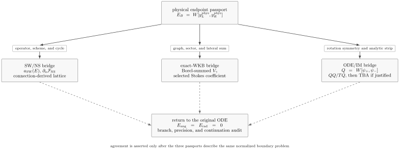
The three lower boxes have different outputs and different existence hypotheses. A common vocabulary such as “quantum period” does not identify them. For a fixed problem, a branch exists only when its gate can be derived. Each candidate must return to the same selected angular and radial Wronskians.

The minimum passport for each route is:

Bridge	Added data	Primary computed object	What can vanish
SW/NS	Quantum operator, gauge theory, mass shifts, $U(1)$ scheme, Seiberg–Witten electric–magnetic cycle, logarithm branch	$a_{\mathrm{SW}}(E)$ and $\partial_{a_{\mathrm{SW}}}\mathcal F_{\mathrm{NS}}$	A boundary-derived exponential combination, not a bare period in every convention
Exact WKB	Formal $\hbar$ embedding, square-root sheet, Stokes graph, continuation path, lateral/median sum	Borel-summed Voros symbol $V_\gamma$	The selected entry of an ordered product of Stokes and Voros matrices
ODE/IM	Discrete rotations, normalized canonical solutions, spectral cover, analyticity strip, divisor	Normalized Wronskian/$Q$-function and its functional relations	A designated $Q$-function; the TBA is a later inversion

Two routes may describe the same operator yet use inequivalent analytic completions. Matching the classical spectral curve or the first few formal period coefficients does not settle that question.

The Kerr SW/NS route starts from a connection coefficient

For nonextremal asymptotically flat Kerr, write the rotation parameter as $a_{\mathrm K}$ and reserve $a_{\mathrm{SW}}$ for the Coulomb/quantum A-period. With time dependence $\ee^{-\ii\omega t}$,

$$r_\pm = M\pm\sqrt{M^2-a_{\mathrm K}^2}, \qquad \Omega_H = \frac{a_{\mathrm K}}{2Mr_+}, \qquad T_H = \frac{r_+-r_-}{8\pi Mr_+}.$$

The separated spin-$s$ Teukolsky angular and radial equations are confluent Heun equations. Here the connection-formula convention uses $s=0,-1,-2$ and a shared angular eigenvalue $\lambda$. Both operators map to the NS limit of $SU(2)$ gauge theory with three fundamental hypermultiplets, but their parameter dictionaries and boundary cycles differ.

Define the instanton and full NS free energies in the scheme used below by

$$\mathcal F_{\mathrm{inst}} = \lim_{\epsilon_2\to0} \epsilon_2 \log Z_{\mathrm{inst}}^{SU(2)} \bigm|_{\epsilon_1=1},$$

and

$$\mathcal F_{\mathrm{full}} = \mathcal F_{\mathrm{class}} +\mathcal F_{\text{1-loop}} +\mathcal F_{\mathrm{inst}}.$$

At $\epsilon_1=1$, the logarithmic derivative meant by this scheme is

$$\begin{aligned} \partial_{a_{\mathrm{SW}}}\mathcal F_{\mathrm{full}} ={}&-2a_{\mathrm{SW}}\log\Lambda +2\log\frac{\Gamma(1+2a_{\mathrm{SW}})} {\Gamma(1-2a_{\mathrm{SW}})} \\ &+ \sum_{j=1}^{3} \log\frac{\Gamma(1/2+m_j-a_{\mathrm{SW}})} {\Gamma(1/2+m_j+a_{\mathrm{SW}})} +\partial_{a_{\mathrm{SW}}}\mathcal F_{\mathrm{inst}}. \end{aligned}$$

All logarithms are continued from a declared weak-coupling branch. An integer shift caused by circling a Gamma divisor changes the lifted lattice label, even though the underlying exponential condition is unchanged.

The Matone coordinate is

$$E = a_{\mathrm{SW}}^2 -\Lambda\partial_\Lambda \mathcal F_{\mathrm{inst}},$$

which must be inverted on a chosen branch to obtain $a_{\mathrm{SW}}(E)$. The symbol $E$ here is a quantum-curve accessory coordinate, not the boundary function $E_B$.

The angular sector fixes the Coulomb branch

Set $c=a_{\mathrm K}\omega$. In the displayed $U(1)$ scheme, the angular dictionary is

$$\lambda = \lambda_s-s,$$

where $\lambda_s$ is the eigenvalue used on the first two pages of this chapter. Thus $\lambda(0)=\ell(\ell+1)-s(s+1)$; omitting this crosswalk would shift both the angular and radial dictionaries.

$$\begin{aligned} \Lambda_{\mathrm a}&=4c, & (m_1,m_2,m_3)_{\mathrm a} &=(-m,-s,-s), \\ E_{\mathrm a} &= \frac14+c^2+s(s+1)-2cs+\lambda. \end{aligned}$$

Regularity at both axes selects

$$a_{\mathrm{SW,a}} = \ell+\frac12, \qquad \ell\ge\max(|m|,|s|),$$

after the resonant endpoint limit is assembled. Equivalently,

$$\lambda-\lambda_0 = 2cs-c^2 -\left. \Lambda\partial_\Lambda \mathcal F_{\mathrm{inst}} \left( \Lambda,\ell+\frac12,-m,-s,-s \right) \right|_{\Lambda=4c},$$

where $\lambda_0=\ell(\ell+1)-s(s+1)$. This is the angular equation that must accompany the radial frequency condition.

The radial sector fixes a selected NS lattice

The radial $SU(2)$ masses and scale are

$$\begin{aligned} \Lambda_{\mathrm r} &=-2\ii\omega(r_+-r_-), \\ m_1^{\mathrm r} &= -\frac{\ii(\omega-m\Omega_H)}{2\pi T_H} +2\ii M\omega, \\ m_2^{\mathrm r} &=-2\ii M\omega-s, \\ m_3^{\mathrm r} &=-2\ii M\omega+s. \end{aligned}$$

The radial accessory coordinate is

$$\begin{aligned} E_{\mathrm{SW,r}} ={}& \frac14+\lambda+s(s+1) +a_{\mathrm K}^2\omega^2 -8M^2\omega^2 \\ &- \left(2M\omega^2+\ii s\omega\right) (r_+-r_-). \end{aligned}$$

Irregular conformal-block crossing gives the horizon-ingoing solution at infinity as a sum of outgoing and incoming canonical waves. In the chosen normalization, its unwanted incoming coefficient has the form

$$C_{\mathrm{in}}^{\mathrm{NS}} = \mathcal N_{\mathrm r} \left[ 1- \exp\!\left( \partial_{a_{\mathrm{SW}}} \mathcal F_{\mathrm{full}} \right) \right], \qquad \mathcal N_{\mathrm r}\ne0,$$

on a generic meromorphic chart. This excludes $\Lambda=0$, resonant $2a_{\mathrm{SW}}\in\mathbb Z$, Gamma divisors, zeros or poles introduced by normalized conformal blocks, Matone branch points, and coalescing endpoint bases. Therefore, within that chart,

$$C_{\mathrm{in}}^{\mathrm{NS}}=0 \quad\Longleftrightarrow\quad \partial_{a_{\mathrm{SW}}} \mathcal F_{\mathrm{full}} = 2\pi\ii k, \qquad k\in\mathbb Z,$$

with

$$a_{\mathrm{SW}} = a_{\mathrm{SW}}(E_{\mathrm{SW,r}})$$

on the branch connected to the desired mode. This is a connection-derived condition: the boundary flag precedes the period lattice.

Do not splice two printed lattices

Another common convention writes the same Kerr/Schwarzschild rule as $\Pi_B=2\pi(n+1/2)$. At $\epsilon_1=1$, a compatible crosswalk between the Aminov–Grassi–Hatsuda (AGH) period convention and the Bonelli–Iossa–Panea Lichtig–Tanzini (BILT) convention used here is

$$\begin{aligned} \Lambda_{\mathrm{AGH}}&=4\Lambda_{\mathrm{BILT}}, & a_{\mathrm{AGH}}&=\ii a_{\mathrm{BILT}}, \\ E_{\mathrm{AGH}} &=-E_{\mathrm{BILT}} +\frac12m_3\Lambda_{\mathrm{BILT}}, \\ \Pi_B^{\mathrm{AGH}} &= \ii\partial_{a_{\mathrm{BILT}}} \mathcal F_{\mathrm{BILT}}-\pi. \end{aligned}$$

Hence the AGH half-integer lattice maps to an integer BILT lattice after the mode label is relabeled. The two formulas also differ by a $U(1)$ shift and may permute the three masses. Convert the full connection coefficient—or compare the resulting normal-form operator—not only the right-hand side.

At an excluded divisor the factored expression may look like $0/0$ or $0\cdot\infty$. Return to the unfactored connection coefficient and take the resonant limit before deciding whether a physical zero is present.

At finite instanton order, solving the angular equation and radial lattice produces a candidate pair $(\lambda,\omega)$. Its status becomes physical only when the original angular-regular and horizon-ingoing/infinity-outgoing Wronskians both vanish. The nonextremal formula also cannot be evaluated at $r_+=r_-$ by direct substitution: the $N_f=3$ data undergo a correlated decoupling to an $N_f=2$ quantum curve.

Extremal Reissner–Nordström exposes the exact-WKB gate

A recent, especially transparent exact-WKB laboratory is a massless scalar on four-dimensional extremal Reissner–Nordström. Its present status should be read narrowly: the derivation and high-order tests apply to the scalar extremal problem and a fixed Stokes topology, not yet to generic nonextremal or gravitational perturbations.

At $Q=M$, the metric function is

$$f(r)=\left(1-\frac Mr\right)^2.$$

After

$$r=M(1+z), \qquad \phi(r)=\left(1+\frac1z\right)\psi(z),$$

the radial equation becomes the doubly confluent Heun equation

$$\left[ -\frac{\dd^2}{\dd z^2} -(M\omega)^2 \left(1+\frac1z\right)^4 +\frac{\ell(\ell+1)}{z^2} \right]\psi(z)=0.$$

Both $z=0$ and $z=\infty$ are irregular. On the positive real ray, the event-ingoing and infinity-outgoing boundary lines are

$$\psi(z) \sim \begin{cases} \exp(\ii M\omega/z)\, z^{1-2\ii M\omega}, & z\to0^+, \\ \exp(\ii M\omega z)\, z^{2\ii M\omega}, & z\to+\infty. \end{cases}$$

The formal Planck parameter is part of the dictionary

The physical equation contains no small parameter. Exact WKB therefore requires an $\hbar$-embedding, and infinitely many embeddings are possible. The source fixes one through the $SU(2)$, $N_f=2$ quantum Seiberg–Witten curve:

$$\left[ -\hbar^2\frac{\dd^2}{\dd z^2} +Q_0(z) +\hbar^2Q_2(z) \right]\psi(z)=0,$$

with

$$\begin{aligned} Q_0(z) ={}& \frac{\Lambda^2}{z^4} +\frac{2m_2\Lambda}{z^3} -\frac{2u}{z^2} +\frac{2m_1\Lambda}{z} +\Lambda^2, \\ Q_2(z) ={}&-\frac1{4z^2}. \end{aligned}$$

The physical operator is recovered by

$$\begin{aligned} \hbar&=1, & \Lambda&=-\ii M\omega, & m_1=m_2&=-2\ii M\omega, \\ 2u&= 6(M\omega)^2 -\left(\ell+\frac12\right)^2. \end{aligned}$$

Then

$$Q_0(z) = -(M\omega)^2 \left(1+\frac1z\right)^4 +\frac{(\ell+1/2)^2}{z^2},$$

while $Q_2$ converts the Langer-shifted $(\ell+1/2)^2$ back to $\ell(\ell+1)$ in the full operator. Treating $\hbar$ as a bookkeeping symbol without this $Q_2$ term would define a different quantum problem.

For

$$\mathcal A=\frac{\ell+1/2}{M\omega},$$

the four simple turning points are

$$\begin{aligned} \alpha_\pm &= \frac{-\mathcal A-2 \pm\sqrt{\mathcal A(\mathcal A+4)}}{2}, \\ \beta_\pm &= \frac{\mathcal A-2 \pm\sqrt{\mathcal A(\mathcal A-4)}}{2}. \end{aligned}$$

The discriminant values $\mathcal A=0,\pm4$ are excluded from the simple-turning- point analysis. The source finds the same graph topology at its sampled parameter values away from these discriminants, but explicitly assumes rather than proves that topology globally.

Use the traditional exact-WKB logarithmic derivative $S^{\mathrm{trad}}$ defined by

$$\hbar^2 \left[ (S^{\mathrm{trad}})^2 +\partial_zS^{\mathrm{trad}} \right] =Q_0+\hbar^2Q_2,$$

and let $S_{\mathrm{odd}}^{\mathrm{trad}}$ denote its sheet-odd formal solution. In the notation of the exact-WKB chapters, $S_{\mathrm{odd}}^{\mathrm{trad}}=P_{\mathrm{even}}/\hbar$. Choose the square-root branch so that, after Borel summation,

$$\Psi_-(z) \sim \exp(\ii M\omega/z)z^{1-2\ii M\omega}$$

near $z=0^+$, while

$$\Psi_+(z) \sim \exp(\ii M\omega z)z^{2\ii M\omega}$$

near positive infinity. The sign labels are fixed by these asymptotics; they are not synonyms for dominant and subdominant on every Stokes curve.

Two Stokes crossings produce the unwanted coefficient

Let $\beta_-$ and $\beta_+$ be the two turning points encountered by the declared continuation from region I near the horizon to region III near infinity. For the source’s branch-cut and counterclockwise orientation, the connection is

$$\begin{aligned} \begin{pmatrix} \Psi_+^{\mathrm I} \\ \Psi_-^{\mathrm I} \end{pmatrix} ={}& \begin{pmatrix} 1&0 \\ -\ii&1 \end{pmatrix} \begin{pmatrix} V_\gamma^{1/2}&0 \\ 0&V_\gamma^{-1/2} \end{pmatrix} \\ &\times \begin{pmatrix} 1&\ii \\ 0&1 \end{pmatrix} \begin{pmatrix} \Psi_+^{\mathrm{III}} \\ \Psi_-^{\mathrm{III}} \end{pmatrix}, \end{aligned}$$

where

$$V_\gamma = \exp\!\left[ \mathcal S_\vartheta \oint_\gamma S_{\mathrm{odd}}^{\mathrm{trad}}(z)\,\dd z \right].$$

The cycle $\gamma$ surrounds $\beta_-$ and $\beta_+$ counterclockwise, and $\mathcal S_\vartheta$ is the Borel sum in the declared direction. Reading the second row gives

$$\begin{aligned} \Psi_-^{\mathrm I} ={}& -\ii V_\gamma^{1/2} \Psi_+^{\mathrm{III}} \\ &+ \left( V_\gamma^{1/2} +V_\gamma^{-1/2} \right) \Psi_-^{\mathrm{III}}. \end{aligned}$$

The first term is the desired infinity-outgoing line. The companion branch $\Psi_-^{\mathrm{III}}$ carries the unwanted infinity-incoming asymptotic

$$\Psi_-^{\mathrm{III}} \sim \exp(-\ii M\omega z)z^{-2\ii M\omega}.$$

Taking a Wronskian with the outgoing branch gives

$$\begin{aligned} W[\Psi_-^{\mathrm I},\Psi_+^{\mathrm{III}}] ={}& \left(V_\gamma^{1/2}+V_\gamma^{-1/2}\right) \\ &\times W[\Psi_-^{\mathrm{III}},\Psi_+^{\mathrm{III}}]. \end{aligned}$$

The last Wronskian is nonzero because the region-III pair is a fundamental frame. Hence the radial boundary function is, up to a nonzero endpoint normalization,

$$E_{\mathrm{rad}}^B \propto V_\gamma^{1/2} +V_\gamma^{-1/2}.$$

It follows that

$$E_{\mathrm{rad}}^B=0 \quad\Longleftrightarrow\quad V_\gamma=-1,$$

or, on a chosen logarithm lift,

$$\mathcal S_\vartheta \oint_\gamma S_{\mathrm{odd}}^{\mathrm{trad}}(z)\,\dd z = 2\pi\ii \left(n+\frac12\right), \qquad n\in\mathbb Z.$$

This derivation is stronger than guessing a Bohr–Sommerfeld lattice: it identifies the exact connection entry whose vanishing produces the lattice.

Borel–Padé computes an approximation to the bridge

For high-order computation it is convenient to rescale the quantum-curve parameters. The homogeneous transformation

$$\begin{aligned} (\hbar,\Lambda,m_1,m_2,u) \longmapsto{}& (\kappa\hbar,\kappa\Lambda, \kappa m_1,\kappa m_2,\kappa^2u) \end{aligned}$$

leaves the operator unchanged up to an overall nonzero factor. Taking $\kappa=\Lambda_{\mathrm{old}}^{-1}=\ii/(M\omega)$ gives

$$\hbar=\frac{\ii}{M\omega}, \qquad \Lambda=1, \qquad m_1=m_2=2, \qquad 2u=-6+\frac{(\ell+1/2)^2}{(M\omega)^2}.$$

Writing the corresponding period as

$$\Pi_B(\hbar) = \sum_{k=0}^{\infty} \hbar^{2k}\Pi_B^{(k)},$$

the coefficient convention is

$$\Pi_B^{(k)} = \ii\oint_\gamma S_{2k-1}(z)\,\dd z, \qquad S_{\mathrm{odd}}^{\mathrm{trad}} = \sum_{k\ge0}\hbar^{2k-1}S_{2k-1}.$$

For the same counterclockwise $\gamma$, $\Pi_B=\ii\hbar\oint_\gamma S_{\mathrm{odd}}^{\mathrm{trad}}\dd z$. The earlier logarithmic condition therefore becomes

$$\mathcal S_0\Pi_B = -2\pi\hbar\left(n+\frac12\right).$$

The source prints the equivalent plus-sign version after the relabeling $\widetilde n=-n-1$. Its ordinary even Borel transform and positive-ray sum are

$$\widehat\Pi_B(\zeta) = \sum_{k=0}^{\infty} \frac{\Pi_B^{(k)}}{(2k)!}\zeta^{2k}$$

and

$$\mathcal S_0\Pi_B = \int_{0}^{\infty} \ee^{-\zeta} \widehat\Pi_B(\hbar\zeta)\,\dd\zeta,$$

when the ray is nonsingular. Replacing $\widehat\Pi_B$ by a Padé approximant defines $\mathcal S_0^{[M/N]}\Pi_B$, not the exact sum. A reliable computation must vary $(M,N)$, inspect Padé-pole condensation, and use lateral sums when singularities meet the ray.

The 2026 extremal-scalar study computes 160 quantum corrections and finds about ten-digit agreement for its best-tested extremal Reissner–Nordström fundamental mode. That is strong numerical evidence for the resummed condition in the tested chamber, while the finite Borel–Padé residual remains an error estimator rather than a theorem of global Borel summability.

For $\ell=0$ and the source’s relabeled fundamental index $\widetilde n=0$, it reports

$$M\omega = 0.133458893567069 -0.095843842128115\ii,$$

with a $[160/160]$ normalized quantization residual

$$\Delta_{\widetilde n}^{[M/N]} = \frac{\mathcal S_0^{[M/N]}\Pi_B}{2\pi\hbar} -\left(\widetilde n+\frac12\right)$$

of approximately $3.4\times10^{-10}$.

The same Stokes topology and condition apply to the scalar extremal Kerr examples studied there after a different parameter identification. However, the corotating $m=\ell>0$ sector changes topology and is excluded from that claim; generic nonextremal, electromagnetic, and gravitational extensions remain separate problems.

The D3-brane ODE/IM function is a canonical Wronskian

The cleanest black-hole-adjacent ODE/IM example begins with an extremal D3-brane scalar. After separation on the transverse sphere, its radial normal form is

$$\frac{\dd^2\phi}{\dd r^2} + \left[ \omega^2\left(1+\frac{L^4}{r^4}\right) - \frac{(\ell+2)^2-\frac14}{r^2} \right]\phi=0.$$

Use

$$r=L\ee^{y/2}, \qquad \phi=\ee^{y/4}\psi, \qquad \omega L=-2\ii\ee^\theta, \qquad P=\frac{\ell+2}{2}.$$

The equation becomes a generalized modified-Mathieu problem,

$$-\frac{\dd^2\psi}{\dd y^2} + \left[ \ee^{2\theta} \left(\ee^y+\ee^{-y}\right) +P^2 \right]\psi=0.$$

The logarithm $\theta$ lives on a cover because $\omega L=-2\ii\ee^\theta$. Its sheet is part of the QNM passport.

Let $\psi_{+,0}$ and $\psi_{-,0}$ be the canonically normalized subdominant solutions at $y\to+\infty$ and $y\to-\infty$, respectively. Their leading normalization is

$$\begin{aligned} \psi_{+,0} &\sim \frac{\ee^{-\theta/2-y/4}}{\sqrt2} \exp\!\left[-2\ee^{\theta+y/2}\right], \\ \psi_{-,0} &\sim \frac{\ee^{-\theta/2+y/4}}{\sqrt2} \exp\!\left[-2\ee^{\theta-y/2}\right]. \end{aligned}$$

Define the normalized central Wronskian

$$Q(\theta,P) = W\!\left[ \psi_{+,0},\psi_{-,0} \right].$$

The Liouville gauge preserves its zero divisor exactly. Indeed,

$$W_r[\phi_1,\phi_2] = \frac2L W_y[\psi_1,\psi_2].$$

What still requires care is the choice of solution lines. In the book’s $\ee^{-\ii\omega t}$ convention, substituting $\omega L=-2\ii\ee^\theta$ into the displayed recessive asymptotics gives, on their real-$y$ rays,

$$\phi_+ \sim\ee^{-\ii\omega r}, \qquad \phi_- \sim r\ee^{-\ii\omega L^2/r}.$$

These are the time-reflected phases of the physical outgoing and ingoing lines used on the preceding pages. Thus “regular” here means canonical subdominant in an ODE/IM Stokes sector. For the published Bethe-root claim to equal the book’s physical Wronskian, those canonical lines must be continued to the physical sectors. The cited paper does not display this phase reconciliation; the zero-set identification is instead strongly supported by its numerical comparisons. If the continuation maps each endpoint line up to a nonzero scalar, then locally

$$E_{\mathrm{rad}}^B(\omega) = g(\theta,P)Q(\theta,P), \qquad g\ne0,$$

and the QNMs are the Bethe roots

$$Q(\theta_n,P)=0$$

on the physical frequency sheet. The nonzero factor $g$ records the difference between the gravitational and ODE/IM endpoint normalizations.

Discrete rotations close a QQ relation

The modified-Mathieu operator has enough discrete rotation symmetry to generate neighboring canonical solutions. Wronskian identities then give

$$Q\!\left(\theta+\frac{\ii\pi}{2}\right) Q\!\left(\theta-\frac{\ii\pi}{2}\right) = 1+Q(\theta)^2.$$

At a QNM root,

$$Q\!\left(\theta_n+\frac{\ii\pi}{2}\right) Q\!\left(\theta_n-\frac{\ii\pi}{2}\right) =1.$$

The accompanying $TQ$ identity is

$$T(\theta)Q(\theta) = Q\!\left(\theta-\frac{\ii\pi}{2}\right) + Q\!\left(\theta+\frac{\ii\pi}{2}\right).$$

At $Q(\theta_n)=0$, it says that the two shifted values are opposite. Combining this with their product being one gives

$$\begin{aligned} Q\!\left(\theta_n+\frac{\ii\pi}{2}\right) &=\sigma\ii, \\ Q\!\left(\theta_n-\frac{\ii\pi}{2}\right) &=-\sigma\ii, \qquad \sigma\in\{+1,-1\}. \end{aligned}$$

In particular, both shifted $Y$-values equal $-1$. This deduction uses no division by $Q(\theta_n)$.

This relation is exact at the functional-equation level in the displayed normalization. A different normalization $Q\mapsto h(\theta)Q$ changes the constant term unless $h$ satisfies the corresponding cocycle equation.

Setting $Y=Q^2$ produces

$$Y\!\left(\theta+\frac{\ii\pi}{2}\right) Y\!\left(\theta-\frac{\ii\pi}{2}\right) = \left[1+Y(\theta)\right]^2.$$

The $Y$-system alone does not determine $Y$. To invert it, one must fix a branch of $\log Y$, the large-$\theta$ drive, the $\theta\to-\infty$ asymptotic, and a strip free of unrecorded zeros and poles.

The TBA is an analytic inversion, not another definition of Q

On the ground-state analytic sheet, let

$$\varepsilon(\theta,P)=-\log Y(\theta,P).$$

With the source normalization, the integral equation is

$$\begin{aligned} \varepsilon(\theta) ={}& \frac{16\pi^{3/2}}{\Gamma(1/4)^2}\, \ee^\theta \\ &- 2\int_{-\infty}^{\infty} \frac{ \log\!\left(1+\ee^{-\varepsilon(\theta')}\right) }{ \cosh(\theta-\theta') } \frac{\dd\theta'}{2\pi}. \end{aligned}$$

The angular label is supplied through the second asymptotic condition

$$\varepsilon(\theta,P) \sim 8P\theta, \qquad \theta\to-\infty.$$

After analytic continuation from the real axis to $\zeta_n=\theta_n-\ii\pi/2$, $Q(\theta_n)=0$ is equivalent to

$$Y\!\left(\theta_n-\frac{\ii\pi}{2}\right)=-1,$$

or

$$\varepsilon\!\left( \theta_n-\frac{\ii\pi}{2} \right) = -\ii\pi(2n+1), \qquad n=0,1,2,\ldots,$$

with the logarithm lift tracked continuously.

Under the stated analytic and nonzero assumptions, the real-line TBA admits continuation in the open strip $|\operatorname{Im}\theta|<\pi/2$. For finite modes on the positive-$\operatorname{Re}\omega$ branch, $\zeta_n$ lies inside its lower half. In the high-overtone limit it approaches the lower edge, where a lateral or residue prescription is required. In the final 2025 journal convention, the exponential map lets each overtone be represented on an appropriate logarithm sheet within this strip. Selected $n=0,1$ modes are checked against Leaver data. For example, at $L=1$, $\ell=1$, and $n=0$, the reported values are

$$\begin{aligned} \omega_{\mathrm{TBA}}L &=2.09176-0.50175\ii, \\ \omega_{\mathrm{Leaver}}L &=2.09176-0.50181\ii. \end{aligned}$$

For $\ell=25$, the same computation follows the branch through $n=3000$ and approaches $\omega_nL\sim-1.85407(n+1/2)\ii$. Large-$n$ numerical instability is reported, and the high-overtone comparison is to this asymptotic law rather than to an independent Leaver value at every $n$.

The equal-charge subfamily is extremal Reissner–Nordström in isotropic coordinates, and a multicomponent $QQ/Y/TBA$ system has been constructed for the broader four-charge family. That does not establish an ODE/IM closure for every Kerr, de Sitter, or AdS equation. The discrete rotation orbit and analytic strip must be derived anew.

The four-charge example makes this failure of universality visible. Let $\Sigma_j$ be the elementary symmetric charge combinations, with $\Sigma_4$ fixed. In gravity variables, one of its functional relations is

$$\begin{aligned} &Y\!\left( \theta+\frac{\ii\pi}{2}; -\ii\Sigma_1,-\Sigma_2,\ii\Sigma_3 \right) \\ &\quad\times Y\!\left( \theta-\frac{\ii\pi}{2}; -\ii\Sigma_1,-\Sigma_2,\ii\Sigma_3 \right) \\ &= \left[1+Y(\theta;\Sigma_1,\Sigma_2,\Sigma_3)\right] \left[1+Y(\theta;-\Sigma_1,\Sigma_2,-\Sigma_3)\right]. \end{aligned}$$

A rapidity shift therefore rotates the gravitational charge data. This is a coupled relation across analytically continued geometries, not a scalar $Y$-system at one fixed black hole. Equal charges recover the extremal Reissner–Nordström subfamily in isotropic coordinates; the unequal-charge family should not be renamed Reissner–Nordström.

Agreement requires eight matching gates

The three bridges can be compared only after they have been reduced to the same normalization-complete boundary problem. A practical equivalence manifest has eight rows:

Gate	Question that must have the same answer
Operator	Do the scalar gauges and coordinate changes give exactly the same differential operator, including $Q_2$, Langer, and accessory terms?
Spectral cover	Are frequency, rapidity, Coulomb modulus, and logarithm sheets related by one explicit map?
Endpoint flags	Which one-dimensional solution lines are ingoing, outgoing, regular, Dirichlet, or subdominant after continuation?
Normalization	Are the endpoint frames related by holomorphic units, and have every Gamma or sine divisor and resonant limit been recorded?
Cycles	Which oriented homology classes, intersection pairing, and electric–magnetic basis define the periods?
Analytic completion	Is a formal NS/WKB series, a lateral Borel sum, a canonical Wronskian, or a TBA solution being compared?
Chamber	How do Stokes mutations, charge rotations, and branch crossings act along the chosen continuation path?
Spectral divisor	Do the functions have the same zeros with multiplicity, and do those zeros satisfy the original angular and radial boundary equations?

Passing only the operator gate is common and insufficient. For example, the extremal Reissner–Nordström exact-WKB construction derives a Voros condition, but it does not derive the D3-brane Baxter $Q$, its $QQ$ relation, or its nonlinear integral equation. Conversely, a $1/\cosh(\theta-\theta')$ kernel in two resummation problems does not identify their cycles, endpoint normalizations, or analytic continuations.

One model-specific NS/ODE–IM crosswalk

For the pure-$SU(2)$ D3-brane problem—not for Kerr—the final 2025 journal normalization uses

$$\omega L=-2\ii\frac{\Lambda_0}{\hbar}, \qquad \frac18(\ell+2)^2=\frac{u}{\hbar^2},$$

and states

$$Q(a,\Lambda_0,\hbar) = \ii\, \frac{ \sin\!\left[A_D(a,\Lambda_0,\hbar)/\hbar\right] }{ \sin(2\pi a/\hbar) }, \qquad A_D=\partial_a\mathcal F.$$

Away from denominator zeros, $Q=0$ gives $A_D(a,\Lambda_{0,k},\hbar)=\pi k\hbar$. At a correlated numerator and denominator zero, this quotient cannot determine the divisor without a limit. Older preprint conventions use hyperbolic functions and different factors of $\ii$; they must not be spliced into this sine formula.

The shared invariant is therefore not the printed period. It is the selected boundary line and its unwanted connection coefficient. Periods, Voros symbols, and $Q$-functions are coordinate systems for that invariant only after all eight gates close.

A reproducible computation returns to the original ODE

Use the bridge as a candidate generator and the physical Wronskians as the certificate.

1. Fix the passport. Record the time dependence, frequency sheet, endpoint sectors, angular convention, and continuation path. Store $a_{\mathrm K}$ and $a_{\mathrm{SW}}$ under different variable names.
2. Build a seeded pair. Start at a limit with known angular and radial data. For Kerr, solve the angular Matone equation and the radial NS equation simultaneously; never insert an arbitrary separation constant into the radial condition and call the result a QNM.
3. Evaluate one declared representation. In the NS route, vary instanton order and monitor the Matone branch. In exact WKB, vary the quantum-period order, Padé degrees, Borel direction, and graph chamber. In ODE/IM, vary the real-line cutoff, mesh, nonlinear iteration tolerance, logarithm branch, and strip-edge continuation.
4. Continue rather than reseed. Track the root as one physical parameter changes. Monitor a scaled Jacobian and its singular-value gap; a sudden jump may be a branch switch rather than a new mode.
5. Evaluate independent boundary functions. Integrate or recur from both physical endpoints and compute $E_{\mathrm{ang}}$ and $E_{\mathrm{rad}}^B$ at one or more matching points. Rescale the endpoint solutions independently to verify that only a nonzero factor changes.
6. Certify convergence. Demand stable digits under increased precision, displaced matching points, altered truncations, and a second numerical representation such as continued fractions. Report normalized residuals, not only agreement with a printed frequency.

A raw residual or Jacobian condition number changes when either boundary function is multiplied by a nonzero factor. Choose positive output scales $\rho_{\mathrm{ang}},\rho_{\mathrm{rad}}$ and input scales $s_A,s_\omega$, and record

$$\begin{aligned} \boldsymbol F &= \begin{pmatrix} E_{\mathrm{ang}}\\ E_{\mathrm{rad}}^B \end{pmatrix}, & D_{\mathrm{out}} &= \operatorname{diag} (\rho_{\mathrm{ang}}^{-1},\rho_{\mathrm{rad}}^{-1}), \\ D_{\mathrm{in}} &= \operatorname{diag}(s_A,s_\omega). \end{aligned}$$

Here $A$ has returned to the chapter’s physical separation constant; the Reissner–Nordström turning-point ratio was $\mathcal A$. Define

$$\begin{aligned} \widetilde{\boldsymbol F} &=D_{\mathrm{out}}\boldsymbol F, & \widetilde J &= D_{\mathrm{out}} \partial_{(A,\omega)}\boldsymbol F D_{\mathrm{in}}, \\ \widetilde R_{\mathrm{ang}} &=|\widetilde F_1|, & \widetilde R_{\mathrm{rad}} &=|\widetilde F_2|, \\ \kappa_{\widetilde J} &= \frac{\sigma_{\max}(\widetilde J)} {\sigma_{\min}(\widetilde J)}. \end{aligned}$$

The scales are part of the acceptance record. If an endpoint solution is renormalized, its output scale must change with it. Small scaled residuals without stability in $\kappa_{\widetilde J}$ can signal a nearly multiple root. In that case, certify the local intersection multiplicity or topological degree, or use a multidimensional contour count, before assigning mode labels.

Common pitfalls

Quantizing a period before deriving a boundary coefficient. A quantum period is not spectral by itself. Derive the connection entry selected by the physical endpoint lines, then read off the lattice on a declared logarithm branch.

Confusing Kerr rotation with the Coulomb period. The symbols are often both printed as $a$. Keeping $a_{\mathrm K}$ and $a_{\mathrm{SW}}$ distinct prevents dimensionally plausible but incorrect substitutions.

Mixing NS schemes term by term. A rescaling of $\Lambda$, an imaginary Coulomb coordinate, a $U(1)$ factor, or a logarithm shift changes the printed lattice. Translate the complete exponential connection coefficient and its divisors.

Calling a finite Borel–Padé value exact. Exact WKB refers to the Borel-summed connection problem under analytic hypotheses. A finite Padé approximant is numerical evidence; its diagonal sequence, pole pattern, and lateral contour still require an audit.

Reusing a Stokes word across a graph wall. A turning-point collision or active saddle changes the basis and Voros coordinates. The physical Wronskian is preserved only if the connection word is mutated with them.

Deriving a TBA from a $Y$-system alone. Functional relations do not fix zero modes, source terms, logarithm branches, or hidden zeros and poles. Those analytic data are precisely what distinguish a valid inversion from an extra solution of the same $Y$-system.

Reading ODE/IM recession as a physical wave without continuation. The D3 real-$y$ canonical solutions carry the time-reflected phases in the book convention. Match the time sign, frequency sheet, and Stokes sectors before identifying their Wronskian with a Green-function denominator.

Validating a representation with itself. Agreement between two instanton truncations or two Padé degrees is an internal convergence test, not an independent physical check. Evaluate the original endpoint Wronskians or a separately derived recurrence.

Exercises

1. Recover the modified-Mathieu equation and its Wronskian

Starting from the D3 radial equation, use $r=L\ee^{y/2}$ and $\phi=\ee^{y/4}\psi$ to derive the displayed modified-Mathieu equation. Show also that $W_r[\phi_1,\phi_2]=(2/L)W_y[\psi_1,\psi_2]$.

Solution

Since $\partial_r=(2/r)\partial_y$,

$$\frac{\dd^2\phi}{\dd r^2} = \frac4{r^2} \left( \frac{\dd^2\phi}{\dd y^2} -\frac12\frac{\dd\phi}{\dd y} \right).$$

Substitution of $\phi=\ee^{y/4}\psi$ cancels the first derivative and gives

$$-\psi'' + \left[ -\frac{(\omega L)^2}{4} (\ee^y+\ee^{-y}) +\frac{(\ell+2)^2}{4} \right]\psi=0.$$

Using $\omega L=-2\ii\ee^\theta$ and $P=(\ell+2)/2$ gives the equation on the page. For two solutions, the derivative of the common gauge factor cancels in the determinant:

$$\begin{aligned} W_r[\phi_1,\phi_2] &=\frac2rW_y[\ee^{y/4}\psi_1,\ee^{y/4}\psi_2] \\ &=\frac2r\ee^{y/2}W_y[\psi_1,\psi_2] =\frac2L W_y[\psi_1,\psi_2]. \end{aligned}$$

2. Multiply the extremal Reissner–Nordström connection word

Multiply the three exact-WKB matrices and recover the coefficient of $\Psi_-^{\mathrm{III}}$ in $\Psi_-^{\mathrm I}$. Why is its zero equivalent to $V_\gamma=-1$?

Solution

The product is

$$\begin{pmatrix} V_\gamma^{1/2}&\ii V_\gamma^{1/2} \\ -\ii V_\gamma^{1/2}& V_\gamma^{1/2}+V_\gamma^{-1/2} \end{pmatrix}.$$

The second row therefore gives the continuation printed above. The unwanted incoming coefficient is $V_\gamma^{1/2}+V_\gamma^{-1/2}$. A Voros symbol is an exponential and is nonzero, so multiplying by $V_\gamma^{1/2}$ reduces its zero condition to $V_\gamma+1=0$.

3. Derive the shifted Bethe-root condition without dividing by Q

At $Q(\theta_n)=0$, combine the $QQ$ and $TQ$ relations to prove that the two shifted $Y$-values equal $-1$.

Solution

Write

$$q_+=Q\!\left(\theta_n+\frac{\ii\pi}{2}\right), \qquad q_-=Q\!\left(\theta_n-\frac{\ii\pi}{2}\right).$$

The $QQ$ relation gives $q_+q_-=1$, while $TQ$ at the root gives $q_++q_-=0$. Hence $q_-=-q_+$ and $-q_+^2=1$. Therefore $q_+^2=q_-^2=-1$, which is precisely $Y(\theta_n\pm\ii\pi/2)=-1$.

4. Audit the Kerr angular eigenvalue convention

The earlier chapter convention has $\lambda_s(0)=\ell(\ell+1)-s^2$. Show that $\lambda=\lambda_s-s$ gives the seed required by the NS dictionary.

Solution

At $c=0$,

$$\lambda(0) = \ell(\ell+1)-s^2-s = \ell(\ell+1)-s(s+1).$$

This is $\lambda_0$ in the displayed instanton formula. Because the radial accessory contains the same $\lambda$, the conversion must be made before either sector is evaluated.

5. Translate the two NS lattices

Use $\Pi_B^{\mathrm{AGH}} =\ii\partial_a\mathcal F_{\mathrm{BILT}}-\pi$ to map $\Pi_B^{\mathrm{AGH}}=2\pi(n+1/2)$ to the BILT integer lattice.

Solution

Substitution gives

$$\ii\partial_a\mathcal F_{\mathrm{BILT}}-\pi =2\pi n+\pi.$$

Thus

$$\partial_a\mathcal F_{\mathrm{BILT}} =-2\pi\ii(n+1).$$

This has the BILT form $2\pi\ii k$ after the relabeling $k=-n-1$. The half-integer versus integer appearance is therefore not a physical disagreement.

6. Locate the D3 frequency-sheet audit

Insert $\omega L=-2\ii\ee^\theta$ into the two canonical exponentials. What does $\theta\mapsto\theta+\ii\pi$ do, and why must the endpoint passport record it?

Solution

Because $\ee^\theta=\ii\omega L/2$, the $y\to+\infty$ exponential becomes $\exp(-\ii\omega r)$ and the $y\to-\infty$ exponential becomes $\exp(-\ii\omega L^2/r)$. The shift $\theta\mapsto\theta+\ii\pi$ changes $\ee^\theta$ to $-\ee^\theta$ and therefore sends $\omega$ to $-\omega$ in this parametrization. It reverses both endpoint phases and, after Stokes continuation, selects the opposite canonical lines. It also changes the logarithm sheet and the path through Stokes sectors. Recording only the final value of $\omega$ loses the data needed to decide which physical boundary lines were continued.

7. Design a Borel–Padé reliability test

Give four checks that distinguish a stable numerical Borel–Padé estimate from an unsupported claim of exact summation.

Solution

One should vary the numerator and denominator degrees along several near- diagonal sequences, inspect the Padé poles relative to the Laplace ray, compare upper and lower lateral contours when poles approach that ray, and increase the number of WKB coefficients. The resulting candidate frequency must then be tested against the original endpoint Wronskian. Stability of only one Padé sequence can conceal pole–zero defects or a wrong Stokes chamber.

8. Write an equivalence manifest

Suppose an extremal black-hole DCHE has both a proposed NS period and an exact-WKB Voros condition. List the minimum evidence needed before calling them equivalent.

Solution

Exhibit the identical scalar operator including its $\hbar$ embedding and subleading potential; map every spectral parameter and logarithm sheet; identify the same physical endpoint lines; map the WKB cycle to the electric–magnetic basis with orientation and intersection form; account for all gauge, Gamma, and $U(1)$ normalizations; equate the chosen Borel/NS analytic completions in one chamber; track wall crossings; and show that the two functions equal the same boundary Wronskian up to a holomorphic unit. Finally compare multiplicities and evaluate the original boundary function at representative common zeros. A shared classical curve or matching asymptotic coefficients closes only the first few gates.

References

• G. Aminov, A. Grassi, and Y. Hatsuda, “Black Hole Quasinormal Modes and Seiberg–Witten Theory”, Annales Henri Poincaré 23 (2022), 1951–1977. Proposes the exact quantum-period rules and tests the Schwarzschild and Kerr dictionaries; its radial identification is presented as a conjecture.
• G. Bonelli, C. Iossa, D. Panea Lichtig, and A. Tanzini, “Exact Solution of Kerr Black Hole Perturbations via CFT$_2$ and Instanton Counting: Greybody Factor, Quasinormal Modes, and Love Numbers”, Physical Review D 105 (2022), 044047. Derives the confluent-Heun connection coefficients and the BILT Kerr dictionaries used here.
• G. Bonelli, C. Iossa, D. Panea Lichtig, and A. Tanzini, “Irregular Liouville Correlators and Connection Formulae for Heun Functions”, Communications in Mathematical Physics 397 (2023), 635–727. Develops generic confluent-Heun connection charts and their Stokes-sector choices.
• Y. Hatsuda and T. Shiga, “Exact WKB and Quantum Periods for Extremal Black Hole Quasinormal Modes”, arXiv:2605.01321 (May 2026 preprint). Derives the scalar extremal Reissner–Nordström and selected extremal Kerr Stokes conditions and performs 160-order Borel–Padé tests.
• N. Nikolaev, “Existence and Uniqueness of Exact WKB Solutions for Second-Order Singularly Perturbed Linear ODEs”, Communications in Mathematical Physics 400 (2023), 463–517. Supplies the analytic exact-WKB existence theorem; it does not identify black-hole endpoint flags by itself.
• D. Fioravanti and D. Gregori, “New Method for Exact Results on Quasinormal Modes of Black Holes”, Physical Review D 112 (2025), 125020. Gives the D3-brane and four-charge $Q/QQ/Y/TBA$ constructions and the high-overtone numerical results quoted above.
• D. Fioravanti and D. Gregori, “Integrability and Cycles of Deformed $\mathcal N=2$ Gauge Theory”, Physics Letters B 804 (2020), 135376. Establishes the canonical modified-Mathieu ODE/IM solutions and their gauge-period relations.
• D. Fioravanti, D. Gregori, and H. Shu, “Integrability, SUSY $SU(2)$ Matter Gauge Theories and Black Holes”, Nuclear Physics B 1021 (2025), 117200. Develops the matter-coupled ODE/IM systems, asymptotics, kernels, and gravitational dictionaries.
• M. Bianchi, D. Consoli, A. Grillo, and J. F. Morales, “QNMs of Branes, BHs and Fuzzballs from Quantum SW Geometries”, Physics Letters B 824 (2022), 136837. Gives the physical D3 radial equation, boundary phases, and independent SW, WKB, and Leaver benchmarks.
• K. Imaizumi, “Quasi-Normal Modes for the D3-Branes and Exact WKB Analysis”, Physics Letters B 834 (2022), 137450. Provides a chamber-specific exact-WKB connection derivation and graph-mutation analysis for the D3 equation.