Stokes Sectors, Formal Monodromy, and Wild Monodromy

Ordinary monodromy compresses one circuit around an irregular point into one matrix. Wild monodromy keeps the missing factorization: formal exponential scales, their deck action, direction-labelled Stokes factors, and the connection between local asymptotic frames and a global base frame. This refinement is exactly what asymptotic connection problems need.

The local construction and summability theory were developed in Chapter 1. Here the emphasis is different: we package those local factors as global analytic data, identify the residual normalization group, and show precisely what is lost when only the ordinary monodromy conjugacy class is retained.

Status of the statements

Once normalized sectorial frames exist, the transition, periodicity, and monodromy identities below are exact. Their existence with a prescribed formal asymptotic expansion requires the summability or sectorial hypotheses stated in Chapter 1. The moduli-space language is schematic until the irregular type, marking, and quotient group are fixed.

The puncture becomes a circle of directions

Let $x=0$ be an irregular singularity. After a minimal ramified cover $x=t^p$, a formal fundamental matrix has the schematic form

$$\widehat\Phi(t) = \widehat H(t)\, \ee^{Q(t)}t^\Lambda.$$

The formal package needed below records:

• the ramification and exponential factors in the diagonal or block-diagonal matrix $Q$;
• the regular-singular formal blocks encoded by $\Lambda$ and possible nilpotent terms;
• the deck permutation of the exponential blocks;
• the generalized formal monodromy $M_{\mathrm f}$.

In the wild-character literature, the irregular type means specifically the polar exponential datum $Q$. Formal monodromy is separate from $Q$. A broader formal model may also include the ramification, regular-singular blocks, and their formal return. A moduli problem must say which parts are fixed.

To keep directional asymptotics visible, replace the point $x=0$ by its real oriented blow-up. In polar coordinates

$$x=r\ee^{\ii\theta}, \qquad r\geq0,$$

the new boundary $r=0$ is a circle parametrized by $\theta$. A small sector at the puncture becomes a neighborhood of an arc on this boundary. Canonical sectorial frames live over such arcs, and singular summation directions become marked boundary points.

When $x=t^p$, the exponential factors live first on the $p$-fold cover of this boundary. Its angular coordinates satisfy

$$\theta_x=p\,\theta_t \pmod{2\pi}.$$

Sector frames and exponential labels are indexed on the $t$-boundary before the deck action is used to descend them to the original $x$-circle. Intrinsically, ramified exponential factors form a finite covering, or exponential local system,

$$\mathcal I\longrightarrow\partial\widetilde X.$$

They need not admit one global labelling on the $x$-boundary circle.

For an ordered exponential difference

$$\Delta q_{\alpha\beta} = q_\alpha-q_\beta,$$

this book marks a jump direction by the phase condition that $\exp(\Delta q_{\alpha\beta})$ is maximally small. The equal-magnitude condition

$$\operatorname{Re}\Delta q_{\alpha\beta}=0$$

is different. Naming both kinds of ray “Stokes rays” in different sources is one reason the phase condition, rather than the name, belongs in every normalization ledger.

Sector frames and direction-labelled factors

Choose counterclockwise-indexed sectorial fundamental matrices

$$\Phi_j \sim \widehat H\,\ee^Q t^\Lambda$$

with the same formal normalization. On an overlap, two such matrices differ by a constant:

$$\Phi_{j+1}=\Phi_jS_j.$$

The matrix $S_j$ is the Stokes factor for that oriented crossing. It lies in the unipotent Stokes group selected by the active exponential differences at that direction. In a nonresonant rank-two problem this may be an upper- or lower-triangular one-parameter group; repeated exponential blocks and several slopes require a filtered block group instead.

Two distinctions are essential.

First, $S_j$ compares two canonical normalizations. Continuing one fixed solution frame across the same boundary uses

$$\Phi_j^{\mathrm{cont}} = \Phi_{j+1}S_j^{-1}.$$

Second, the index $j$ includes its lift to the angular cover. A matrix without the oriented direction and lift that label it is not complete Stokes data.

Formal return and actual local monodromy

Suppose one positive circuit in the original $x$-plane crosses $m$ boundaries. Choose the equivariant normalization

$$\Phi_{j+m}=\Phi_jM_{\mathrm f}.$$

It includes the power-factor continuation and any permutation induced by the ramified deck transformation. Comparing

$$\Phi_{j+m+1} = \Phi_{j+m}S_{j+m}$$

with

$$\Phi_{j+1}M_{\mathrm f} = \Phi_jS_jM_{\mathrm f}$$

gives the formal periodicity law

$$S_{j+m} = M_{\mathrm f}^{-1}S_jM_{\mathrm f}.$$

Now continue a fixed basis from sector $0$ through every boundary:

$$\begin{aligned} \Phi_0^{\mathrm{cont}} &= \Phi_1S_0^{-1}\\ &= \Phi_2S_1^{-1}S_0^{-1}\\ &\ \vdots\\ &= \Phi_mS_{m-1}^{-1}\cdots S_0^{-1}. \end{aligned}$$

Using $\Phi_m=\Phi_0M_{\mathrm f}$ yields

$$M_{\mathrm{loc}} = M_{\mathrm f} S_{m-1}^{-1}\cdots S_0^{-1}.$$

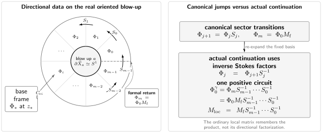
The real oriented blow-up separates asymptotic directions. Canonical frames cross by $S_j$, while a fixed continued frame uses $S_j^{-1}$; after the formal return, their ordered product is $M_{\mathrm{loc}}$.

All three order choices are now visible:

1. sectors are indexed counterclockwise in the declared local coordinate;
2. canonical transitions act on the right;
3. actual continuation uses their inverses in reverse accumulated order.

Changing any one of these conventions changes the printed product.

What “wild monodromy” contains

This book uses wild monodromy data for the full formal, Stokes, and connection package. Some sources use “wild monodromy” more narrowly for the monodromy around one tangential puncture, which becomes a Stokes automorphism after a sectorial splitting is chosen.

For a fixed irregular type, a framed generalized local data set consists schematically of

$$\left( M_{\mathrm f}, S_0,\ldots,S_{m-1} \right),$$

together with the exponential labels, their angular order, and their deck action. To compare this local package with data at other punctures, also choose a path and a connection matrix to the global base frame.

If

$$\Phi_i=\Phi_*C_{*i},$$

then

$$M_i^{(*)} = C_{*i}M_{\mathrm{loc},i}C_{*i}^{-1}.$$

On a punctured sphere, the regular and irregular actual local matrices in the common frame obey

$$M_1^{(*)}\cdots M_N^{(*)}=I.$$

The product constraint uses $M_{\mathrm{loc},i}$, not $M_{\mathrm f,i}$ alone. The Stokes factors have already entered through the local product. Here $C_{*i}$ conjugates a based local automorphism such as the complete $M_{\mathrm{loc},i}$. A raw $S_j$ is instead an arrow between two different sector frames; expressing it globally requires sector-specific connection paths or transport to a common tangential frame.

Two related constructions organize this information:

• A Stokes-filtered local system is the solution local system on the boundary circle together with its filtration indexed by the exponential local system.
• In the unramified topological model, a Stokes local system is an honest local system on an auxiliary tangentially punctured real blow-up. It has a flat reduction to $H_i=C_G(Q_i)$ in each halo, and its monodromy around the tangential puncture in direction $d$ lies in the Stokes group $\operatorname{Sto}_d(Q_i)$. The local system itself does not jump; matrices $S_j$ appear after choosing sectorial splittings or trivializations.

For a reductive group $G$, the corresponding unramified framed Stokes-representation variety is written

$$\operatorname{Hom}_{\mathbb S}(\Pi,G).$$

Here $\Pi$ is the fundamental groupoid of the auxiliary punctured surface with chosen halo base points, and the subscript $\mathbb S$ imposes the Stokes-group conditions at the tangential punctures.

With

$$H=\prod_i C_G(Q_i),$$

the coarse wild character variety is the affine GIT quotient

$$\mathcal M_B(\Sigma) = \operatorname{Hom}_{\mathbb S}(\Pi,G) \mathbin{//}H.$$

Its points are S-equivalence classes, not arbitrary orbit labels. Fixing $H_i$-conjugacy classes of the formal monodromies selects symplectic leaves; smoothness additionally requires stable or generic hypotheses.

This groupoid language prevents a common mistake. There is no single unlabelled “wild matrix” replacing ordinary monodromy; the extra information is a network of formal, sectorial, and connection arrows subject to product relations. Ramified types require the intrinsic exponential-local-system or twisted version of this construction.

A two-factor rank-two calculation

Take

$$S_0=I+s_0E_{12}, \qquad S_1=I+s_1E_{21},$$

and

$$M_{\mathrm f} = \begin{pmatrix} \mu&0\\ 0&\mu^{-1} \end{pmatrix}, \qquad \mu\ne0.$$

With the book’s continuation convention,

$$\begin{aligned} M_{\mathrm{loc}} &= M_{\mathrm f}S_1^{-1}S_0^{-1}\\ &= \begin{pmatrix} \mu&-\mu s_0\\ -\mu^{-1}s_1& \mu^{-1}(1+s_0s_1) \end{pmatrix}. \end{aligned}$$

Two immediate audits are

$$\det M_{\mathrm{loc}}=1$$

and

$$\operatorname{tr}M_{\mathrm{loc}} = \mu+\mu^{-1}(1+s_0s_1).$$

Assume now that $Q$ has two distinct, labelled, one-dimensional exponential blocks and that no block swap is allowed. The centralizer of the irregular type,

$$H=C_{GL(2)}(Q),$$

is then the diagonal torus, represented by

$$D = \operatorname{diag}(d_1,d_2).$$

If a regular-singular formal block is also fixed, the admissible group is its stabilizer inside $H$. Centralizing $M_{\mathrm f}$ alone would be wrong when $\mu^2=1$, because it would allow transformations that do not preserve the distinct exponential grading.

Under the constant formal-frame change

$$S_j\longmapsto D^{-1}S_jD,$$

the multipliers transform as

$$s_0 \longmapsto \frac{d_2}{d_1}s_0, \qquad s_1 \longmapsto \frac{d_1}{d_2}s_1.$$

Thus the product $s_0s_1$ is invariant, while either numerical multiplier alone depends on the framed normalization.

This example also locates exactly where ordinary monodromy loses data. For $s_0s_1\ne0$, the product and fixed $\mu$ determine the generic orbit under this diagonal centralizer. On the divisor $s_0s_1=0$, however, the three Stokes possibilities

$$(s_0,s_1)=(0,0), \qquad (s_0,0), \qquad (0,s_1)$$

with the displayed nonzero entry are distinct direction-labelled data. If $\mu^2\ne1$, all three actual matrices are nevertheless conjugate to the same diagonal semisimple matrix. The ordinary local conjugacy class cannot tell “no jump” from a one-sided jump.

If the formal type admits a symmetry that swaps the two labelled blocks, the last two one-sided orbits may be identified. The quotient group must therefore be fixed before orbit coordinates are interpreted.

There is a second quotient subtlety. Under the diagonal-torus action,

$$\mathbb C[s_0,s_1]^{\mathbb C^*} = \mathbb C[s_0s_1].$$

The two nonzero one-sided orbits are not closed: each closure contains $(0,0)$. Thus all three product-zero orbits define one S-equivalence point in the coarse affine GIT quotient. Their directional distinction survives in the framed data, orbit groupoid, or quotient stack—not as three points of the coarse wild character variety.

Framed versus unframed numbers

A table of numerical Stokes multipliers is framed data. It becomes comparable across papers only after the formal basis, sector order, exponential labels, and centralizer normalization have been translated.

Ramification and several exponential levels

The preceding $2\times2$ calculation is the simplest chart, not the general definition.

Ramified exponential factors

If $x=t^p$, one positive $x$-circuit sends

$$t\longmapsto\ee^{2\pi\ii/p}t.$$

It may permute the exponential factors rather than return each one to itself. The generalized $M_{\mathrm f}$ therefore contains a deck permutation as well as the continuation of $t^\Lambda$. Stokes directions should first be indexed on the cover; descending them prematurely can identify distinct arrows.

Repeated blocks

When several solutions share one exponential factor, the formal centralizer is larger than a diagonal torus. It contains automorphisms of the repeated regular-singular block. Stokes data must be quotiented by this full centralizer, and scalar multiplier coordinates may cease to be natural.

Several slopes

With several positive formal levels, the Stokes group at one direction has a filtration by exponential decay rate. Its element $S_d\in\operatorname{Sto}_d(Q)$ has a unique ordered factorization by levels. Passing to the full $S_d$ loses nothing while $Q$, the direction $d$, and the filtered Stokes group remain attached. Information is lost only if that factor is subsequently treated as an arbitrary unlabelled unipotent matrix.

Coalescing directions

As parameters vary, exponential differences can collide or vanish. Singular directions merge, the formal centralizer jumps, and one coordinate chart on Stokes data may degenerate. A pole in a chosen multiplier can therefore be a normalization singularity rather than a singularity of the underlying family. Confluence requires the parameter-sector and basis control developed in Chapter 1.

A global-data ledger

Before using irregular monodromy in a connection or spectral formula, record:

Layer	Required data
Geometry	Surface, puncture, local coordinate, angular cover, and orientation
Formal type	Ramification, exponential factors, regular blocks, and $M_{\mathrm f}$
Direction data	Phase condition, lifted singular directions, and sector order
Sector frames	Asymptotic normalization and lateral prescription
Stokes factors	Right-transition direction, active block, and multiplier
Global transport	Base point, path, and $C_{*i}$
Actual monodromy	Ordered product and conjugation into the common frame
Quotient	Irregular-type centralizers $H_i=C_G(Q_i)$, stabilizers of any additional fixed formal data, and quotient notion—GIT, stack, or orbit set
Parameters	Coalescence, resonance, vanishing normalization, and chamber exclusions

This ledger distinguishes an exact framed formula from an invariant statement on a wild character variety.

Common pitfalls

Using a Stokes factor in the continuation product without inversion. The equation $\Phi_{j+1}=\Phi_jS_j$ compares canonical sector frames. Continuation of a fixed frame uses $S_j^{-1}$.

Dropping the angular lift. In ramified problems, two rays with the same projection to the $x$-plane may act on different exponential labels. Work on the minimal cover until the deck action has been recorded.

Quotienting only by diagonal matrices. A diagonal centralizer is generic for distinct one-dimensional exponential blocks. Repeated blocks require the full automorphism group of the formal type.

Calling the ordinary product “the wild monodromy.” The product is one shadow of the generalized data. Wild data retain the direction-labelled factorization and its connection to the global frame.

Treating a divergent multiplier as an intrinsic singularity. At coalescence, sector coordinates and canonical bases can fail even when the connection family remains regular on a common punctured domain.

Exercises

1. Derive formal periodicity. Starting from $\Phi_{j+1}=\Phi_jS_j$ and $\Phi_{j+m}=\Phi_jM_{\mathrm f}$, derive the relation between $S_{j+m}$ and $S_j$.

Solution

Compute $\Phi_{j+m+1}$ in two ways:

$$\Phi_{j+m+1} = \Phi_{j+m}S_{j+m} = \Phi_jM_{\mathrm f}S_{j+m},$$

and

$$\Phi_{j+m+1} = \Phi_{j+1}M_{\mathrm f} = \Phi_jS_jM_{\mathrm f}.$$

Cancellation of $\Phi_j$ gives

$$M_{\mathrm f}S_{j+m} = S_jM_{\mathrm f},$$

hence

$$S_{j+m} = M_{\mathrm f}^{-1}S_jM_{\mathrm f}.$$

2. Multiply the two-factor model. Compute $M_{\mathrm f}S_1^{-1}S_0^{-1}$, its determinant, and its trace.

Solution

Since $E_{12}^2=E_{21}^2=0$,

$$S_0^{-1}=I-s_0E_{12}, \qquad S_1^{-1}=I-s_1E_{21}.$$

Therefore

$$S_1^{-1}S_0^{-1} = \begin{pmatrix} 1&-s_0\\ -s_1&1+s_0s_1 \end{pmatrix},$$

and left multiplication by $M_{\mathrm f}$ gives the displayed $M_{\mathrm{loc}}$. Each factor has determinant one, so $\det M_{\mathrm{loc}}=1$. Summing its diagonal entries gives

$$\operatorname{tr}M_{\mathrm{loc}} = \mu+\mu^{-1}(1+s_0s_1).$$

3. Find the residual invariant. For two distinct labelled one-dimensional exponential blocks with no block swap, derive the diagonal-torus action on $s_0,s_1$. Classify its orbits when $s_0s_1\ne0$ and when $s_0s_1=0$.

Solution

For $D=\operatorname{diag}(d_1,d_2)$,

$$D^{-1}E_{12}D = \frac{d_2}{d_1}E_{12}, \qquad D^{-1}E_{21}D = \frac{d_1}{d_2}E_{21}.$$

Thus $s_0s_1$ is invariant. If it is nonzero, choose $d_2/d_1$ to send $s_0$ to any prescribed nonzero value; $s_1$ is then fixed by the product, so each nonzero product is one orbit.

If the product vanishes, there are three orbits:

$$(0,0), \qquad (\mathbb C^*,0), \qquad (0,\mathbb C^*).$$

The last two remember which direction carries the nontrivial jump. They are not closed, however, and all three product-zero orbits map to the same point of the affine GIT quotient.

4. Transport an irregular local product. Let $\Phi_i=\Phi_*C_{*i}$ and suppose $M_{\mathrm{loc},i}=M_{\mathrm f,i}S_{i,1}^{-1}S_{i,0}^{-1}$. Derive the monodromy in the base frame.

Solution

Since $\Phi_*=\Phi_iC_{*i}^{-1}$ on the chosen overlap, continuation around the based local loop gives

$$\begin{aligned} \Phi_*^\gamma &= \Phi_iM_{\mathrm{loc},i}C_{*i}^{-1}\\ &= \Phi_* C_{*i}M_{\mathrm{loc},i}C_{*i}^{-1}. \end{aligned}$$

Therefore

$$M_i^{(*)} = C_{*i} M_{\mathrm f,i} S_{i,1}^{-1}S_{i,0}^{-1} C_{*i}^{-1}.$$

5. Audit a ramified return. Suppose $x=t^3$ and one positive $x$-circuit cyclically permutes three one-dimensional exponential blocks. Explain why a diagonal $M_{\mathrm f}$ in the fixed block order is impossible.

Solution

A positive $x$-circuit sends

$$t\longmapsto\ee^{2\pi\ii/3}t.$$

By hypothesis this sends block $1$ to $2$, $2$ to $3$, and $3$ to $1$. In the original fixed ordering, the formal return must therefore contain the cyclic permutation matrix. Power-factor continuation can multiply its nonzero entries by phases, but it cannot remove the permutation. A diagonal matrix would falsely claim that each exponential block returned to itself.

References

• Y. Sibuya, Linear Differential Equations in the Complex Domain: Problems of Analytic Continuation, AMS, 1990, for canonical sectorial solutions and Stokes multipliers.
• W. Wasow, Asymptotic Expansions for Ordinary Differential Equations, Wiley, 1965; Dover reprint, 1987, for formal solutions, asymptotic sectors, and monodromy.
• W. Balser, Formal Power Series and Linear Systems of Meromorphic Ordinary Differential Equations, Springer, 2000, for formal reduction, summability, and Stokes matrices.
• C. Sabbah, Introduction to Stokes Structures, Springer, 2013, for Stokes-filtered local systems and ramified exponential factors.
• P. P. Boalch, “Topology of the Stokes phenomenon”, for the intrinsic exponential-local-system and Stokes-local-system viewpoints.
• P. P. Boalch, “Geometry and braiding of Stokes data; fission and wild character varieties”, Annals of Mathematics 179 (2014), 301–365, for the unramified Stokes-representation quotient and its Poisson geometry.
• P. P. Boalch, “Poisson varieties from Riemann surfaces”, for a concise geometric overview of wild character data.
• P. P. Boalch and D. Yamakawa, “Twisted wild character varieties”, preprint, for the twisted framework that includes ramified irregular types.