Quantum Wronskians and Exact Quantization

Page 5 derived functional identities that hold for every value of the spectral parameter. None of them, by itself, chooses an energy. The missing operation is geometric: select two one-dimensional spaces of solutions by boundary or recessive-sector conditions, then ask when those two lines coincide.

That distinction is the meaning of exact quantization on this page. “Exact” says that the boundary function is an exact connection Wronskian, not a truncated asymptotic series. It does not promise a closed-form eigenvalue, automatic reality, or a convergent iteration. Nor does it turn a logarithmic functional equation into a thermodynamic Bethe ansatz equation; that requires the analyticity and contour data of Chapter 13.

Continue with the homogeneous radial family

$$\left[ -\frac{\dd^2}{\dd x^2} +x^{2M} +\frac{l(l+1)}{x^2} \right]y =Ey, \qquad M>1,$$

at nonexceptional twist, unless a limiting prescription is stated. Use

$$q=\omega=\ee^{\pi\ii/(M+1)}, \qquad s=v_ME, \qquad \vartheta=2\pi p =\frac{\pi(l+1/2)}{M+1}.$$

The quantization gate

Let $L_A(E)$ and $L_B(E)$ be two declared canonical solution lines and choose nonzero representatives $u_A,u_B$. Their boundary function is

$$F_{AB}(E)=\Wr[u_A,u_B](E).$$

Then

$$F_{AB}(E_*)=0 \quad\Longleftrightarrow\quad L_A(E_*)=L_B(E_*).$$

Thus $E_*$ is spectral precisely when the common line satisfies both declared boundary conditions. For the present ODE:

$$\begin{aligned} Q_+(v_ME,p)=0 &\quad\Longleftrightarrow\quad \text{regular radial boundary problem}, \\ Q_-(v_ME,p)=0 &\quad\Longleftrightarrow\quad \text{alternate radial boundary problem}, \\ T_{n/2}(q^{n-1}v_ME,p)=0 &\quad\Longleftrightarrow\quad \Wr[y_{-1},y_n](E,l)=0, \quad n\geq1, \\ &\quad\Longleftrightarrow\quad \text{recessive in }S_{-1}\text{ and }S_n \text{ at energy }E. \end{aligned}$$

The first two are origin-to-infinity problems. The third is an infinity-to-infinity, or lateral, problem. Equivalently, in the centered coordinate $s$, a zero of $T_{n/2}(s,p)$ represents the raw ODE energy $q^{1-n}s/v_M$. Their zeros must not be mixed.

Status ledger

Statement	Status
A boundary-pair Wronskian vanishes exactly when the two canonical lines coincide	Exact two-dimensional ODE geometry
$Q_+=0$, $Q_-=0$, and $T_{n/2}=0$ encode the three boundary passports displayed above	Exact after the Page 4 scale and normalization dictionary
Positivity and simplicity of regular radial zeros for real $l>-1/2$	Self-adjoint Sturm–Liouville result for the declared Friedrichs domain
The alternate radial zeros form a second self-adjoint spectrum	Only in the limit-circle range of the standing $l>-1/2$ branch and after a second endpoint extension is declared
The radial phase equations below	Exact self-consistency conditions when reality, positivity, genus-zero products, and the continuous phase branch hold
Reality or simplicity of a lateral spectrum	Not automatic; it needs a separate symmetry or spectral theorem
The names Baxter function, Bethe root, and fused transfer function	Model-specific ODE/IM dictionary from Pages 4–5
A TBA or nonlinear integral equation	Requires analyticity strips, zero locations, asymptotics, contours, and logarithm data; deferred to Chapter 13
Identification with an exact-WKB quantization condition	Requires a separate cycle, chamber, and Borel-summation dictionary; not asserted here

A boundary pair, not an all-s identity, quantizes

For a second-order equation in normal form, the solution space at fixed $E$ is two-dimensional. Two nonzero solutions are linearly dependent if and only if their Wronskian vanishes. If $u_A$ spans the solutions allowed at one endpoint or in one Stokes sector and $u_B$ spans those allowed at the other, dependence produces one nonzero solution obeying both conditions. The converse is immediate: any solution satisfying both conditions lies in both one-dimensional lines.

This elementary argument is exact, but its hypotheses carry the physics. A usable boundary passport records the ordered lines, the logarithmic sheet, the contour joining them, the endpoint domain, and the normalizations. Without that passport, $F_{AB}=0$ is only a formal statement.

For the conventions of Pages 2–5, the principal passports are:

Problem	Canonical lines	Boundary function	Spectral meaning
Regular radial	$\langle y_0\rangle$ at infinity and $\langle\psi_+\rangle$ at the origin	$\Delta_-$, hence $Q_+$	$x^{l+1}$ at zero and recessive in $S_0$
Alternate radial	$\langle y_0\rangle$ and $\langle\psi_-\rangle$	$\Delta_+$, hence $Q_-$	$x^{-l}$ at zero and recessive in $S_0$
Lateral $n$	$\langle y_{-1}\rangle$ and $\langle y_n\rangle$	$T_{n/2}(s)$	recessive in both sectors at $E_{\mathrm{ODE}}=q^{1-n}s/v_M$

More explicitly, the centered lateral determinant is

$$\begin{aligned} F_n(s,p) &:=T_{n/2}(s,p) \\ &=\frac{1}{2\ii} \Wr[y_{-1},y_n] \left(q^{1-n}\frac{s}{v_M},l\right), \qquad n\geq0. \end{aligned}$$

The argument shift centers the two sectors in the spectral coordinate; it does not alter the boundary lines. In particular,

$$F_n(s_*,p)=0 \quad\Longleftrightarrow\quad \Wr[y_{-1},y_n](\mathcal E_*,l)=0, \qquad \mathcal E_*=q^{1-n}\frac{s_*}{v_M}.$$

At $n=0$, the lines are adjacent and the Page 2 normalization gives

$$F_0(s,p) =\frac{\Wr[y_{-1},y_0]}{2\ii} =1.$$

Adjacent canonical lines therefore never produce a discrete spectrum. At a finite-cover closure, a more distant pair can instead become the same line for every $E$, making its Wronskian identically zero. That is a global monodromy closure, not a discrete eigenvalue condition. A genuine lateral problem uses distinct, nonadjacent lines and an isolated zero.

The endpoint audit separates the two radial spectra

Take $l$ real and $l>-1/2$. Infinity is limit-point. Near zero, the two Frobenius behaviors have squared magnitudes $x^{2l+2}$ and $x^{-2l}$. Consequently,

$$\begin{array}{c|c|c} \text{range of }l &x^{l+1}\in L^2(0,1) &x^{-l}\in L^2(0,1) \\ \hline -1/2<l<1/2 &\text{yes} &\text{yes} \\ l\geq1/2 &\text{yes} &\text{no} \end{array}$$

Thus zero is limit-circle for $-1/2<l<1/2$ and limit-point for $l\geq1/2$. The regular line $x^{l+1}$ gives the Friedrichs problem for all real $l>-1/2$. Its eigenvalues are positive and simple, and

$$Q_+(v_ME_n^{\mathrm{reg}},p)=0, \qquad n=0,1,2,\ldots.$$

In the limit-circle interval, the alternate line $x^{-l}$ defines a different separated self-adjoint extension, with

$$Q_-(v_ME_n^{\mathrm{alt}},p)=0.$$

Outside that interval, $Q_-$ remains a valuable analytically continued determinant, but its zeros are not automatically a physical half-line spectrum. At $l=0$, the two extensions are familiar: $Q_+$ gives the Dirichlet half-line levels, hence the odd levels of the even full-line potential, while $Q_-$ gives the Neumann and even levels.

The involution $l\mapsto-1-l$ supplies the mirror description for $l<-1/2$: there $x^{-l}$ is the Friedrichs line and the two $Q$-labels exchange roles. Thus the full limit-circle interval is $-3/2<l<1/2$; at $l=-1/2$ the two powers coalesce and one needs the $x^{1/2}$, $x^{1/2}\log x$ basis. The physical naming on this page follows the chosen $l>-1/2$ representative.

The two pure Frobenius lines do not exhaust the limit-circle domains. From

$$(2l+1)y_0 =\Delta_-\psi_- -\Delta_+\psi_+,$$

a mixed endpoint condition $A c_++B c_-=0$ has the raw boundary function

$$F_{A,B}(E) =B\Delta_-(E,l)-A\Delta_+(E,l).$$

In normalized Baxter variables define

$$\begin{aligned} \widehat F_{A,B}(s) &:=F_{A,B}\!\left(\frac{s}{v_M}\right) \\ &=B\Delta_-(0,l)Q_+(s,p) \\ &-A\Delta_+(0,l)Q_-(s,p). \end{aligned}$$

The unequal zero-energy weights are part of the domain data. A generic mixed determinant is not either BLZ $Q$-branch and need not obey either scalar $TQ$ equation. At $l=0$, for example, $\Delta_-=y_0(0)$ and $\Delta_+=-y_0'(0)$. The Robin condition

$$\cos\eta\,y_0(0) +L\sin\eta\,y_0'(0)=0$$

is therefore $\cos\eta\,\Delta_--L\sin\eta\,\Delta_+=0$; Dirichlet and Neumann are the endpoints $\eta=0$ and $\eta=\pi/2$.

A radial zero has a quantum-Wronskian certificate

Write the normalized quantum Wronskian from Page 5 as

$$\begin{aligned} &\ee^{\ii\vartheta} Q_+(qs)Q_-(q^{-1}s) \\ &\quad- \ee^{-\ii\vartheta} Q_+(q^{-1}s)Q_-(qs) =2\ii\sin\vartheta. \end{aligned}$$

The parameters $p$ have been suppressed from the $Q$-arguments. Let $s_i^+$ be a zero of $Q_+$. Substituting first $s=qs_i^+$ and then $s=q^{-1}s_i^+$ gives two denominator-free identities:

$$\begin{aligned} \ee^{\ii\vartheta} Q_+(q^2s_i^+)Q_-(s_i^+) &=2\ii\sin\vartheta, \\ -\ee^{-\ii\vartheta} Q_+(q^{-2}s_i^+)Q_-(s_i^+) &=2\ii\sin\vartheta. \end{aligned}$$

At nonexceptional twist the right-hand side is nonzero. Hence the complementary determinant $Q_-(s_i^+)$ and both shifted $Q_+$ values are nonzero. Eliminating $Q_-(s_i^+)$ recovers

$$\frac{Q_+(q^2s_i^+)} {Q_+(q^{-2}s_i^+)} =-\ee^{-2\ii\vartheta}.$$

Similarly, at $Q_-(s_i^-)=0$,

$$\begin{aligned} -\ee^{-\ii\vartheta} Q_+(s_i^-)Q_-(q^2s_i^-) &=2\ii\sin\vartheta, \\ \ee^{\ii\vartheta} Q_+(s_i^-)Q_-(q^{-2}s_i^-) &=2\ii\sin\vartheta. \end{aligned}$$

Eliminating $Q_+(s_i^-)$ gives

$$\frac{Q_-(q^2s_i^-)} {Q_-(q^{-2}s_i^-)} =-\ee^{2\ii\vartheta}.$$

These are more than root locations: the two un-divided equations certify the normalization of the complementary connection coefficient. They also show that $Q_+$ and $Q_-$ have no common zero at nonexceptional twist. They do not, by themselves, prove that a zero is simple; simplicity in the self-adjoint radial problem comes from Sturm–Liouville theory.

One auxiliary equation contains two boundary problems

Define the meromorphic auxiliary ratios

$$\begin{aligned} a_+(s) &:=\ee^{2\ii\vartheta} \frac{Q_+(q^2s)}{Q_+(q^{-2}s)}, \\ a_-(s) &:=\ee^{-2\ii\vartheta} \frac{Q_-(q^2s)}{Q_-(q^{-2}s)}. \end{aligned}$$

The two $TQ$ equations factor as

$$1+a_\pm(s) =\ee^{\pm\ii\vartheta} \frac{T(s)Q_\pm(s)}{Q_\pm(q^{-2}s)}.$$

Therefore $a_\pm=-1$ can signal either a radial zero of $Q_\pm$ or a lateral zero of $T$, subject to the displayed denominator being nonzero and to possible cancellations. For the standard real ground-state problem, the regular radial roots lie on the positive $E$-axis and the elementary lateral roots lie on a different ray, often represented as the negative axis after the conventional spectral rotation. In a general complex problem, the boundary passport—not the equation $a=-1$—is what separates the two sets.

This is also the precise stopping point before a nonlinear integral equation. Turning $a$ into an NLIE requires a contour that encloses the intended zeros of $1+a$, excludes the other family or includes its source terms, and controls every pole, branch, and asymptotic contribution.

Reality turns the radial ratio into a counting phase

Assume the declared radial problem is self-adjoint, its roots are positive and simple, and the normalized determinant is real on the real axis. Work first in the principal-twist window $|\vartheta|<\pi/2$. Put

$$\phi=\frac{2\pi}{M+1}, \qquad q^{-2}=\ee^{-\ii\phi}.$$

Along the lower rotated ray define a continuous phase, starting at zero,

$$\Theta_\pm(E) :=\Im\Log_{\mathrm{cont}} Q_\pm(q^{-2}v_ME,p), \qquad \Theta_\pm(0)=0.$$

Reality gives

$$Q_\pm(q^2v_ME,p) =\overline{Q_\pm(q^{-2}v_ME,p)}.$$

The radial root relations then become the exact counting conditions

$$\boxed{ \Theta_\pm(E_n^\pm) =\pi\left(n+\frac12\pm2p\right), \qquad n=0,1,2,\ldots }$$

where $E_n^+=E_n^{\mathrm{reg}}$. The minus line is a physical $E_n^{\mathrm{alt}}$ only after the alternate self-adjoint extension has been declared. The displayed equality fixes the continuous branch; a bare principal argument would retain only the equality modulo $\pi$ and would lose the level number.

Outside $|\vartheta|<\pi/2$, the ratio still fixes the phase modulo $\pi$, but the displayed level branch can acquire an integer spectral-flow offset. That integer must be determined by continuous parameter continuation or by the Weyl asymptotics and root ordering; it must not be guessed by reducing $p$ modulo its phase period.

For $M>1$, the genus-zero product makes the self-consistency explicit. If $E_m^\pm$ are the zeros of the selected branch, then

$$Q_\pm(q^{-2}v_ME,p) =\prod_{m=0}^{\infty} \left( 1-\ee^{-\ii\phi}\frac{E}{E_m^\pm} \right).$$

Since $0<\phi<\pi$, every factor has a continuous argument in $(0,\pi)$ for $E>0$. Hence

$$\begin{aligned} \Theta_\pm(E) =\sum_{m=0}^{\infty} \operatorname{atan2}\!\left( \dfrac{E}{E_m^\pm}\sin\phi, 1-\dfrac{E}{E_m^\pm}\cos\phi \right). \end{aligned}$$

Combining this sum with the boxed equation, in its stated twist window, gives a countable system of exact, self-consistent quantization conditions. Large-level asymptotics are still needed to label the solution, determine any spectral-flow offset outside that window, and close a numerical truncation. The equation itself does not prove that a particular fixed-point iteration converges.

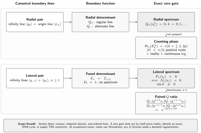
The Page 5 functional identities hold for all $s$. Quantization begins at the solid zero gate after a boundary pair has been declared. The dashed step to a ratio is valid only when its denominator and $\sin(2\pi p)$ are nonzero. Here $s_*$ is the centered fused coordinate; the corresponding raw ODE energy is $q^{1-n}s_*/v_M$.

Fused quantum Wronskians quantize lateral problems

For $n\geq1$, import the fused bilinear from Page 5:

$$\begin{aligned} 2\ii\sin\vartheta\,F_n(s,p) ={}& \ee^{\ii(n+1)\vartheta} Q_+(q^{n+1}s)Q_-(q^{-n-1}s) \\ &- \ee^{-\ii(n+1)\vartheta} Q_+(q^{-n-1}s)Q_-(q^{n+1}s). \end{aligned}$$

Call the right-hand side $\mathcal N_n(s,p)$. At $\sin\vartheta\ne0$, the exact denominator-free lateral condition is

$$F_n(s_*,p)=0 \quad\Longleftrightarrow\quad \mathcal N_n(s_*,p)=0.$$

Only when

$$Q_+(q^{-n-1}s_*)Q_-(q^{n+1}s_*)\ne0$$

may this be written as the paired ratio

$$\frac{ Q_+(q^{n+1}s_*)Q_-(q^{-n-1}s_*) }{ Q_+(q^{-n-1}s_*)Q_-(q^{n+1}s_*) } =\ee^{-2\ii(n+1)\vartheta}.$$

Inserting both canonical products yields

$$\begin{aligned} &\prod_{j=0}^{\infty} \frac{s_j^+-q^{n+1}s_*} {s_j^+-q^{-n-1}s_*} \\ &\quad\times \prod_{k=0}^{\infty} \frac{s_k^--q^{-n-1}s_*} {s_k^--q^{n+1}s_*} =\ee^{-2\ii(n+1)\vartheta}. \end{aligned}$$

This is one complex equation in general. It becomes a real counting-phase condition only on a contour where a conjugation or anti-linear symmetry makes the left-hand side unimodular and a continuous logarithm has been fixed. No such reality claim follows from the fused identity alone.

The case $n=1$ is the elementary lateral determinant $F_1=T$. Setting $T(s_*)=0$ in the two $TQ$ equations gives the two factors of the paired ratio separately. The case $n=0$ is categorically different: $F_0=1$, and the fused formula is the fundamental quantum Wronskian with nonzero right-hand side. It cannot be used as a spectral zero condition.

Quartic audit: three spectra, three labels

For $M=2$ and $l=0$,

$$q=\ee^{\pi\ii/3}, \qquad p=\frac1{12}, \qquad \vartheta=\frac{\pi}{6}.$$

To compare with Voros, note that his determinant uses $(\widehat H+\lambda)\psi=0$, so $\lambda=-E$, with $D_4^-$ Dirichlet and $D_4^+$ Neumann. If

$$j=q^2=\ee^{2\pi\ii/3}, \qquad q^{-2}=j^2,$$

then the precise normalized map is

$$\begin{aligned} Q_+(q^{-2}v_2E) &=\frac{D_4^-(-j^2E)}{D_4^-(0)}, \\ Q_-(q^{-2}v_2E) &=\frac{D_4^+(-j^2E)}{D_4^+(0)}. \end{aligned}$$

The two radial phase equations are

$$\begin{aligned} \Theta_+(E_n^{\mathrm D}) &=\pi\left(n+\frac23\right), \\ \Theta_-(E_n^{\mathrm N}) &=\pi\left(n+\frac13\right). \end{aligned}$$

These are the odd and even full-line quartic levels, respectively. They are not zeros of the elementary lateral determinant. For the lateral $n=1$ problem, $T(s_*)=0$ instead gives

$$\frac{ Q_+(q^2s_*)Q_-(q^{-2}s_*) }{ Q_+(q^{-2}s_*)Q_-(q^2s_*) } =\ee^{-2\pi\ii/3}.$$

Indeed, the two $TQ$ equations at $T=0$ give

$$\begin{aligned} \frac{Q_+(q^2s_*)}{Q_+(q^{-2}s_*)} &=-\ee^{-\pi\ii/3}, \\ \frac{Q_-(q^{-2}s_*)}{Q_-(q^2s_*)} &=-\ee^{-\pi\ii/3}. \end{aligned}$$

Multiplying them produces the fused phase. This check catches both a sign error and the common mistake of using $q^{\pm1}$ rather than $q^{\pm2}$ in the entire variable $s$.

Exceptional twists require a confluent construction

Put $\beta^2=1/(M+1)$ and $\kappa=l+1/2$. The full Frobenius exceptional lattice is

$$\begin{aligned} 2p=\pm(m_1\beta^2+m_2), \qquad m_1,m_2\in\mathbb Z_{\geq0}, \\ \text{equivalently}\qquad \kappa=\pm\bigl[m_1+(M+1)m_2\bigr]. \end{aligned}$$

Its vanishing-prefactor subset is

$$\sin(2\pi p)=0 \quad\Longleftrightarrow\quad 2p\in\mathbb Z.$$

At every point of the full lattice, the normalized $Q$-pair can require regularization even when $\sin\vartheta\ne0$. On the $2p\in\mathbb Z$ subset, division by $\sin\vartheta$ is invalid and the raw boundary Wronskian $F_n$ remains the primary spectral object. At $p=0$, equivalently $l=-1/2$, compatible limits satisfy $Q_+=Q_-$ and the naive normalized quantum Wronskian collapses to $0=0$. Other points with $2p\in\mathbb Z$ require their own limiting audit; the derivative construction below is not a universal regularization of the whole exceptional lattice.

Suppose the regularized branches obey $Q_-(s,p)=Q_+(s,-p)$ and have been constructed along

$$l=\frac{2p}{\beta^2}-\frac12$$

with $M$, hence $q$, fixed. If this family is differentiable at $p=0$, a declared l’Hôpital limit gives

$$F_n(s,0) =\frac{1}{4\pi\ii} \left. \frac{\partial\mathcal N_n(s,p)}{\partial p} \right|_{p=0}.$$

For the fundamental case, write

$$Q_0(s)=Q_+(s,0)=Q_-(s,0), \qquad \dot Q(s)= \left.\partial_pQ_+(s,p)\right|_{p=0}.$$

Differentiating the quantum Wronskian gives the confluent identity

$$\begin{aligned} &Q_0(qs)Q_0(q^{-1}s) \\ &\quad+ \frac{ \dot Q(qs)Q_0(q^{-1}s) -Q_0(qs)\dot Q(q^{-1}s) }{2\pi\ii} =1. \end{aligned}$$

The derivative branch replaces the second solution lost when the two twists coalesce. This formula is conditional on the stated regularized limit. It does not select the critical endpoint domain: at $l=-1/2$ one must still prescribe the coefficient relation between $x^{1/2}$ and $x^{1/2}\log x$. At other points of the Page 4 exceptional lattice, logarithmic Frobenius solutions and normalization poles can require a different confluent basis; one must not extrapolate the displayed $p=0$ formula without checking that basis.

What exact quantization does—and does not—supply

The hierarchy of claims is now sharp:

1. Canonical ODE solutions define exact boundary Wronskians.
2. A declared pair of boundary lines turns an isolated Wronskian zero into a spectral value.
3. Functional relations express that zero using rotated radial determinants.
4. Reality and a continuous logarithm turn a complex ratio into a numbered phase equation.
5. Product and large-energy data turn the phase equation into a self-consistent computational system.

Steps 1–3 are algebraic and analytic consequences of the ODE setup. Step 4 is conditional on the spectral symmetry. Step 5 still needs asymptotic control and a numerical scheme. Page 7 changes the potential; Page 8 audits analyticity and failure modes systematically; Chapter 13 adds the contour deformations that produce TBA and NLIE representations.

Common pitfalls

Quantizing an identity. A $TQ$ or quantum-Wronskian relation valid for every $s$ does not select a level. Name the two canonical boundary lines and set their own Wronskian to zero.

Dividing before checking zeros. The denominator-free bilinear remains valid when a shifted $Q$ vanishes. A ratio is an equivalent condition only after its denominator has been proved nonzero.

Calling every unit-looking ratio a phase. A complex ratio becomes a real phase equation only after conjugation or another anti-linear symmetry proves unit modulus and a continuous logarithm branch is fixed.

Mixing radial and lateral roots. The same equation $1+a=0$ can contain zeros of both $Q$ and $T$. The boundary passport and the root contour, not the auxiliary equation alone, identify the spectrum.

Using a resonant normalization generically. At $\sin(2\pi p)=0$, a normalized bilinear can collapse. Retain the raw Wronskian or construct an explicit confluent limit before taking zeros.

Exercises

1. Prove the zero gate. Let $L_A$ and $L_B$ be one-dimensional subspaces of a two-dimensional solution space. Prove that $\Wr[u_A,u_B]=0$ if and only if a nonzero solution satisfies both line conditions.

Solution

For a second-order normal-form equation, the Wronskian of two solutions vanishes exactly when they are linearly dependent. Dependence means $u_A=c\,u_B$ with $c\ne0$, so their common span belongs to both lines. Conversely, a nonzero solution in $L_A\cap L_B$ spans each one-dimensional space, so $u_A$ and $u_B$ are dependent and their Wronskian vanishes.

2. Classify the endpoint. For real $l>-1/2$, determine when each Frobenius behavior is square-integrable at zero and recover the limit-circle interval.

Solution

The regular behavior obeys

$$\int_0^1x^{2l+2}\,\dd x<\infty \quad\Longleftrightarrow\quad l>-\frac32,$$

which holds in the stated range. The alternate behavior obeys

$$\int_0^1x^{-2l}\,\dd x<\infty \quad\Longleftrightarrow\quad l<\frac12.$$

Both are square-integrable for $-1/2<l<1/2$, so zero is limit-circle there. For $l\geq1/2$, only the regular line is square-integrable and zero is limit-point.

3. Certify a regular root. Starting from the fundamental quantum Wronskian, derive both un-divided identities at a zero $s_i^+$ and prove that $Q_-(s_i^+)\ne0$ when $\sin\vartheta\ne0$.

Solution

Substitute $s=qs_i^+$ and use $Q_+(s_i^+)=0$ to obtain

$$\ee^{\ii\vartheta} Q_+(q^2s_i^+)Q_-(s_i^+) =2\ii\sin\vartheta.$$

Substitution of $s=q^{-1}s_i^+$ gives

$$-\ee^{-\ii\vartheta} Q_+(q^{-2}s_i^+)Q_-(s_i^+) =2\ii\sin\vartheta.$$

The common right-hand side is nonzero, so none of the three factors on the left can vanish. In particular $Q_-(s_i^+)\ne0$.

4. Recover the continuous phase. In the principal-twist window, use reality to derive the radial phase condition from $a_\pm(E_n^\pm)=-1$. Explain why a principal argument is insufficient and what changes outside that window.

Solution

Put $F_\pm=Q_\pm(q^{-2}v_ME_n^\pm)=|F_\pm|\ee^{\ii\Theta_\pm}$. Reality makes the numerator of the shifted ratio $\overline{F_\pm}$. Thus

$$a_\pm(E_n^\pm) =\ee^{\pm2\ii\vartheta} \ee^{-2\ii\Theta_\pm} =-1.$$

Hence

$$\Theta_\pm =\pi\left(n+\frac12\right) \pm\vartheta =\pi\left(n+\frac12\pm2p\right),$$

where continuity from $E=0$, root ordering, and the Weyl tail fix the integer. A principal argument only records this relation modulo $2\pi$, or the root ratio modulo $\pi$, and therefore cannot retain $n$. Outside $|\vartheta|<\pi/2$, an integer spectral-flow offset must be fixed by continuation or by root ordering and Weyl asymptotics.

5. Write the product quantization system. Insert the genus-zero product into $\Theta_\pm(E)$ and state why the series of arguments converges for $M>1$.

Solution

Each factor gives

$$\arg_{\mathrm{cont}} \left(1-\ee^{-\ii\phi}\frac{E}{E_m^\pm}\right) =\operatorname{atan2}\!\left( \frac{E}{E_m^\pm}\sin\phi, 1-\frac{E}{E_m^\pm}\cos\phi \right).$$

Summing and evaluating at $E=E_n^\pm$ gives the boxed phase condition. The determinant order is $\mu=(M+1)/(2M)<1$, so $E_m^\pm\asymp m^{1/\mu}$ and $\sum_m1/E_m^\pm$ converges. The argument sum therefore converges absolutely in its tail.

6. Derive the fused lateral condition. Set $F_n(s_*)=0$ in the fused quantum Wronskian, derive the paired ratio, and list the two conditions needed before calling it a phase equation.

Solution

At nonexceptional twist, $F_n(s_*)=0$ makes the two bilinear terms equal. If the denominator is nonzero, division gives

$$\frac{ Q_+(q^{n+1}s_*)Q_-(q^{-n-1}s_*) }{ Q_+(q^{-n-1}s_*)Q_-(q^{n+1}s_*) } =\ee^{-2\ii(n+1)\vartheta}.$$

Besides denominator nonvanishing, a phase equation needs an anti-linear symmetry that makes the left side unimodular on the selected contour and a continuous logarithm branch that fixes its integer.

7. Audit the quartic phases. For $M=2$, $l=0$, compute the regular, alternate, and elementary lateral phases.

Solution

Here $p=1/12$ and $\vartheta=\pi/6$. Therefore

$$\Theta_+(E_n^{\mathrm D}) =\pi\left(n+\frac23\right), \qquad \Theta_-(E_n^{\mathrm N}) =\pi\left(n+\frac13\right).$$

For the elementary lateral problem $n=1$, the fused phase is

$$\ee^{-2\ii(n+1)\vartheta} =\ee^{-2\pi\ii/3}.$$

These label three different boundary problems even though all are built from the same ODE family.

8. Take the confluent limit. Assuming a differentiable regularized family at $p=0$, derive the displayed derivative quantum Wronskian.

Solution

Use $Q_-(s,p)=Q_+(s,-p)$ and differentiate the normalized quantum Wronskian at fixed $M$. At $p=0$, both branches become $Q_0$. The derivative of the left side is

$$\begin{aligned} 4\pi\ii Q_0(qs)Q_0(q^{-1}s) +2\bigl[ \dot Q(qs)Q_0(q^{-1}s) -Q_0(qs)\dot Q(q^{-1}s) \bigr], \end{aligned}$$

while the derivative of $2\ii\sin(2\pi p)$ is $4\pi\ii$. Division by $4\pi\ii$ gives the stated confluent identity.

References

• Y. Sibuya, Global Theory of a Second Order Linear Ordinary Differential Equation with a Polynomial Coefficient, North-Holland, 1975, for canonical sectorial solutions, Stokes multipliers, and two-sector boundary problems for polynomial coefficients. Its theorems support the infinity-side framework used here, not the inverse-square Frobenius resonance or every branched noninteger-power extension.
• A. Voros, “Exact resolution method for general 1D polynomial Schrödinger equation”, Journal of Physics A 32 (1999), 5993–6007, for self-consistent exact quantization systems built from spectral determinants and their rotated Wronskian identities; see also the corrigendum, Journal of Physics A 33 (2000), 5783–5784.
• A. Voros, “Exercises in Exact Quantization”, Journal of Physics A 33 (2000), 7423–7450, for the homogeneous phase conditions, parity-resolved determinants, and Airy and quartic checks.
• V. Bazhanov, S. Lukyanov, and A. Zamolodchikov, “Spectral Determinants for Schrödinger Equation and Q-Operators of Conformal Field Theory”, Journal of Statistical Physics 102 (2001), 567–576, for the generic-twist radial determinants and normalized quantum Wronskian. Relative to Dorey–Tateo and this page, that paper interchanges the $D^\pm$ labels, reverses the sign of the energy argument, and sets $D^\pm(0)=1$. Thus its normalized $D^+$ is the regular branch called raw $D_-$ by Dorey–Tateo and $Q_+$ on this page.
• P. Dorey and R. Tateo, “On the Relation between Stokes Multipliers and the T–Q Systems of Conformal Field Theory”, Nuclear Physics B 563 (1999), 573–602, with erratum, Nuclear Physics B 603 (2001), 581, for radial and fused lateral spectral determinants, quantum Wronskians, exceptional twists, and the auxiliary zero equation used here.
• P. Dorey, C. Dunning, and R. Tateo, “The ODE/IM Correspondence”, Journal of Physics A 40 (2007), R205–R283, especially Sections 4.1–5.5 and Appendices D–E for the boundary-problem dictionary and the extra analytic hypotheses needed before functional relations become integral equations.