Excited States, Contour Deformation, and Wall Crossing

A ground-state TBA is not discarded when its parameters are continued. Its contour is transported with the analytic solution. If a logarithmic singularity crosses that contour, returning the contour to its reference position creates an explicit source and a new root condition. If instead a kernel pole crosses because two period phases rotate through $\pi/2$, a residue changes the equation and can force a larger set of unknowns. In exact-WKB/BPS examples that enlargement can encode a genuine wall crossing, but the three mechanisms are not synonyms.

This page derives each operation with its orientation visible. The excited-state prototype is the Dorey–Tateo analytic continuation of the scaling Lee–Yang TBA. The wall-crossing prototype is the $A_2$ polynomial Schrödinger problem of Ito–Mariño–Shu: after the first phase wall, the minimal two-cycle equation closes as a three-charge system containing $\gamma_{12}=\gamma_1+\gamma_2$. The final section reconciles that residue calculation with the inverse-jump Kontsevich–Soibelman pentagon used in Chapter 9.

Status ledger

Passage	Status on this page
Source from a crossed zero or pole	Exact contour identity under the displayed primitive, endpoint, branch, and finite-crossing hypotheses
Excited root condition	Exact self-consistency condition; its integer is fixed by continuation
Scaling Lee–Yang one-particle equation	Published model-specific analytic continuation, not a universal formula for every TBA
Scaling Lee–Yang observable residue	Exact for the same transported contour and normalization as the sourced pseudoenergy
Phase-shifted minimal polynomial TBA	Exact in the IMS normalization while adjacent phase differences stay below $\pi/2$
First $A_2$ kernel-pole residues	Published continuation for the stated path $\phi_2-\phi_1>\pi/2$
Three-charge closure	Published change of variables in that wall-crossed chamber
Ordered pentagon identity	Exact algebra in the book’s inverse-jump convention
Equality of a kernel-pole event and BPS mutation	Model-dependent; it requires a geometric charge and index dictionary
All excited states arise by ground-state continuation	False; continuation preserves superselection data unless more seeds are supplied
Numerical root tracking and error control	Deferred to Page 6

Four events require four separate ledgers

The following distinctions prevent most sign and scope errors.

Event	What moves?	What changes in the equation?	What need not change?
Solution monodromy	Parameters circle a branch point	Possibly only the chosen solution branch	Contour and formula can remain unchanged
Excited-state crossing	A zero or pole of $1+\ee^{-\varepsilon_a}$ crosses an integration contour	A source primitive and a root quantization condition	Fusion graph and BPS indices
Kernel-pole crossing	A pole of $K_{ab}$ crosses while a phase or strip is continued	A residue evaluation of $L_b$	It does not alone prove a new BPS state exists
BPS wall crossing	Central-charge rays reorder and the active spectrum mutates	Charge set, indices, and a refactorized RH/TBA description	The ordered sector automorphism and continued physical coordinate

An important fifth possibility is a pinch: singularities approach a contour from opposite sides so that no local deformation avoids both. A pinch is typically a branch point in parameter space. Circling it can produce solution monodromy before any singularity crosses the final reference contour.

Keep four ledgers during any continuation:

1. the divisor ledger of zeros, poles, multiplicities, and branch integers;
2. the contour ledger of orientations, banks, kernel poles, and winding numbers;
3. the chamber ledger of charges, phases, BPS indices, and ordered products;
4. the observable ledger of determinant, period, energy, and boundary normalization.

Changing one ledger does not silently update the others.

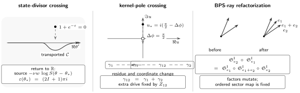
Three continuation events. A crossed nonlinear divisor changes the state passport; a crossed kernel pole changes the contour representation; a BPS wall changes the charge factorization while preserving the ordered sector automorphism. In an established exact-WKB model the last two can describe the same continuation, but that identification is additional structure.

A crossed logarithmic zero produces a source primitive

Write a multi-node equation on transported contours $\mathcal C_b$ as

$$\varepsilon_a(\theta) = d_a(\theta) - \sum_b \int_{\mathcal C_b} K_{ab}(\theta-\theta') L_b(\theta')\,\dd\theta',$$

where

$$L_b(\theta) = \Log z_b(\theta), \qquad z_b(\theta) = 1+\ee^{-\varepsilon_b(\theta)}.$$

Assume that the kernel has a scattering primitive in the chosen strip,

$$K_{ab}(u) = \frac{1}{2\pi\ii} \frac{\dd}{\dd u} \Log S_{ab}(u).$$

This is a convention, not a consequence of the word “TBA.” A matrix Fourier kernel can be treated similarly by first defining a local primitive $\chi_{ab}$ with $\partial_u\chi_{ab}=2\pi\ii K_{ab}$.

Suppose $z_b$ has isolated zeros and poles $\theta_{bj}$ between $\mathcal C_b$ and the reference real line. Let

$$\nu_{bj} = \operatorname{ord}_{\theta_{bj}}z_b$$

be positive for a zero and negative for a pole. Define $w_{bj}$ as the winding number of $\mathcal C_b-\mathbb R$ around $\theta_{bj}$, positive for a counterclockwise loop. Since

$$\partial_{\theta'}L_b(\theta') \sim \frac{\nu_{bj}}{\theta'-\theta_{bj}},$$

integration by parts and the residue theorem give

$$\boxed{ \begin{aligned} \varepsilon_a(\theta) ={}& d_a(\theta) - \sum_b \int_{\mathbb R} K_{ab}(\theta-\theta') L_b(\theta')\,\dd\theta' \\ &- \sum_{b,j} \nu_{bj}w_{bj} \Log S_{ab}(\theta-\theta_{bj}). \end{aligned} }$$

The formula assumes that endpoint terms vanish or are already included in $d_a$, and that no singularity of $S_{ab}$ is crossed during the contour homotopy. It is deliberately orientation-complete: reversing the path changes $w_{bj}$ and hence the source sign. Memorizing an unsigned “$+\log S$ per root” rule is unsafe.

If $z_b$ has a simple zero at $\theta_{bj}$, the source position is not a free parameter. It obeys

$$1+\ee^{-\varepsilon_b(\theta_{bj})}=0,$$

or

$$\varepsilon_b(\theta_{bj}) = (2I_{bj}+1)\pi\ii, \qquad I_{bj}\in\mathbb Z.$$

The integer is branch and state data fixed by continuous tracking. Solving the sourced integral equation while holding a guessed root fixed does not solve the excited-state problem; the integral equation and all root conditions form one coupled nonlinear system.

One pair of roots calibrates the excited-state sign

For the scaling Lee–Yang model, Dorey and Tateo use

$$\varepsilon(\theta) = r\cosh\theta - \phi*L(\theta),$$

with

$$\begin{aligned} L(\theta) &= \log(1+\ee^{-\varepsilon(\theta)}), \\ \phi(\theta) &= -\ii\partial_\theta\log S(\theta), \\ (\phi*L)(\theta) &= \int_{\mathbb R} \frac{\dd\theta'}{2\pi} \phi(\theta-\theta')L(\theta'). \end{aligned}$$

After a particular analytic continuation, two logarithmic singularities lie at $-\theta_0$ and $+\theta_0$. Their transported contour winds counterclockwise around $-\theta_0$ and clockwise around $+\theta_0$. Thus

$$w(-\theta_0)=1, \qquad w(+\theta_0)=-1,$$

and the sourced equation is

$$\boxed{ \begin{aligned} \varepsilon(\theta) ={}& r\cosh\theta + \Log\frac{ S(\theta-\theta_0) }{ S(\theta+\theta_0) } - \phi*L(\theta). \end{aligned} }$$

On the continuously selected one-particle branch,

$$\varepsilon(\theta_0)=\pi\ii.$$

Evaluating the equation at the root gives the companion condition

$$0 = r\cosh\theta_0 - \Log S(2\theta_0) - \phi*L(\theta_0),$$

with the logarithm branch inherited from the continuation. More general one-particle branches allow $\varepsilon(\theta_0)=(2n+1)\pi\ii$ and, away from the spin-zero sector, conjugate rather than reflection-paired roots.

Straightening the contour must also be done in every observable built from $L$. In the normalization of Dorey and Tateo, the effective scaling function changes from its ground-state integral to

$$\begin{aligned} c_{\mathrm{exc}}(r) ={}& \frac{12r\ii}{\pi}\sinh\theta_0 + \frac{3}{\pi^2} \int_{\mathbb R} r\cosh\theta\,L(\theta)\,\dd\theta. \end{aligned}$$

The first term is the residue of the same crossed pair. Adding sources to the pseudoenergy while retaining the old energy or determinant formula would therefore mix two different contour passports.

This example makes two limitations concrete. First, a ground-state formula can acquire a physically excited solution by monodromy before any zero crosses the real line. Second, analytic continuation cannot jump between arbitrary superselection sectors. In the Lee–Yang example, a parity-symmetric seed does not generate nonzero-spin states without an appropriately asymmetric sourced system.

For the Page 2 ODE/IM equations, the same logic applies to whichever nonlinear factor the passport declares. In the fused convention the crossing divisor is $1+Y_a^{-1}=0$; in the DDV convention it is $1+a=0$. The latter has

$$a(\theta_j)=-1, \qquad \Log a(\theta_j)=(2I_j+1)\pi\ii.$$

Which lip of the DDV keyhole is crossed fixes the source sign. A fused root, a DDV hole, and a zero of a spectral determinant are related only after the Page 1 unknown and divisor dictionaries are applied.

A mass phase drives a kernel pole through the contour

Return to the minimal polynomial-potential equation of Page 4. Write

$$m_a=|m_a|\ee^{\ii\phi_a},$$

and shift the real-axis functions by

$$\widetilde\varepsilon_a(\theta) = \varepsilon_a(\theta-\ii\phi_a), \qquad \widetilde L_a(\theta) = L_a(\theta-\ii\phi_a).$$

The phase-shifted kernel is

$$K_{a,b}(u) = \frac{1}{ 2\pi\cosh\!\left( u+\ii(\phi_b-\phi_a) \right) }.$$

The residue-free minimal equation is valid while

$$|\phi_b-\phi_a|<\frac{\pi}{2}$$

for every adjacent pair. The full pole set satisfies

$$u+\ii(\phi_b-\phi_a) = \pi\ii\left(n+\frac12\right), \qquad n\in\mathbb Z.$$

The nearest pair lies at $\pm\pi\ii/2$ before the phase shift. Thus a pole first reaches the real $u$-axis at relative phase $\pm\pi/2$. Either equality is a contour singularity, not a point at which one simply evaluates the old formula. The continuation below follows the positive crossing.

For the $A_2$ chain, put

$$\Delta=\phi_2-\phi_1, \qquad \eta=\Delta-\frac{\pi}{2}.$$

Continue along the IMS path from $\Delta<\pi/2$ to $\eta>0$. With the published lateral prescription, restoring both contours to the real line gives

$$\begin{aligned} \widetilde\varepsilon_1(\theta) ={}& |m_1|\ee^\theta -K_{1,2}*\widetilde L_2(\theta) -\widetilde L_2(\theta+\ii\eta+\ii0), \\ \widetilde\varepsilon_2(\theta) ={}& |m_2|\ee^\theta -K_{2,1}*\widetilde L_1(\theta) -\widetilde L_1(\theta-\ii\eta-\ii0). \end{aligned}$$

These signs are for increasing $\Delta$ in the IMS pseudoenergy and bank convention. Reversing the path reverses the crossed residues. Translating to Page 3’s plus-left inverse-jump convention additionally applies the bank involution fixed on Page 4; one must not mix the two sign ledgers.

The equations are no longer closed on real-axis values: their sources sample $L_1,L_2$ on displaced lines. One can keep those off-axis values as auxiliary unknowns, or change coordinates so the new active charge is explicit.

A composite charge closes the wall-crossed A₂ system

The geometric $A_2$ continuation contains the composite cycle

$$\gamma_{12}=\gamma_1+\gamma_2.$$

In the alternating IMS mass convention,

$$m_{12}=m_1-\ii m_2 = |m_{12}|\ee^{\ii\phi_{12}}.$$

This is simply central-charge addition expressed after the parity-dependent phase choices; it is not a universal formula for arbitrary mass conventions. Introduce the wall-crossed coordinates

$$\begin{aligned} Y_1^{\mathrm n}(\theta) &= \frac{ Y_1(\theta) }{ 1+Y_2(\theta-\frac{\pi\ii}{2}) }, \\ Y_2^{\mathrm n}(\theta) &= \frac{ Y_2(\theta) }{ 1+Y_1(\theta+\frac{\pi\ii}{2}) }, \\ Y_{12}^{\mathrm n}(\theta) &= \frac{ Y_1(\theta)Y_2(\theta-\frac{\pi\ii}{2}) }{ 1+Y_1(\theta)+Y_2(\theta-\frac{\pi\ii}{2}) }. \end{aligned}$$

Set $\varepsilon_a^{\mathrm n}=-\log Y_a^{\mathrm n}$, shift each new function by its mass phase, and then suppress the superscript $\mathrm n$. With

$$K_{a,b}^{\pm}(u) = K_{a,b}\!\left(u\pm\frac{\pi\ii}{2}\right),$$

the closed system is

$$\begin{aligned} \widetilde\varepsilon_1 ={}& |m_1|\ee^\theta -K_{1,2}*\widetilde L_2 -K_{1,12}^{+}*\widetilde L_{12}, \\ \widetilde\varepsilon_2 ={}& |m_2|\ee^\theta -K_{2,1}*\widetilde L_1 -K_{2,12}*\widetilde L_{12}, \\ \widetilde\varepsilon_{12} ={}& |m_{12}|\ee^\theta -K_{12,1}^{-}*\widetilde L_1 -K_{12,2}*\widetilde L_2. \end{aligned}$$

The third pseudoenergy is not an arbitrary numerical stabilizer. It is the coordinate of a definite composite charge with a definite classical drive. In this model, the kernel-pole residue, the new WKB discontinuity, and the enlarged BPS spectrum are three descriptions of one geometric continuation.

For a degree-$(r+1)$ polynomial, the minimal chamber has $r$ adjacent cycles. The maximal chamber can contain

$$\frac{r(r+1)}{2}$$

cycles joining all ordered pairs of turning points. Intermediate chambers have intermediate charge sets. The count is a result for this polynomial geometry; it is not the node count of an arbitrary GMN problem.

The ordered product survives while its factors mutate

Let $e_1\mathbin{\cdot}e_2=1$. In the book’s inverse-jump convention, the elementary automorphisms act on $x=\mathcal V_{e_1}$ and $y=\mathcal V_{e_2}$ by

$$\begin{aligned} \mathfrak S_{e_1}^{\mathrm I} &: (x,y) \longmapsto \left(x,\frac{y}{1+x}\right), \\ \mathfrak S_{e_2}^{\mathrm I} &: (x,y) \longmapsto \left(x(1+y),y\right). \end{aligned}$$

With the rightmost map acting first, the pentagon identity is

$$\boxed{ \mathfrak S_{e_2}^{\mathrm I} \circ \mathfrak S_{e_1}^{\mathrm I} = \mathfrak S_{e_1}^{\mathrm I} \circ \mathfrak S_{e_1+e_2}^{\mathrm I} \circ \mathfrak S_{e_2}^{\mathrm I} }.$$

Both sides send the generators to

$$\left( x(1+y), \frac{y}{1+x+xy} \right).$$

The identity says that the ordered automorphism of a convex sector is unchanged when the two active rays swap order, provided the composite factor is inserted. It does not say that individual coordinates have no Stokes jumps, nor does the algebra by itself prove that a proposed ODE has the required active charges. That geometric input comes from its WKB spectral network or BPS structure.

The relation to the integral equation can now be stated precisely:

• a contour residue is an analytic fact about a chosen representation;
• a charge mutation is discrete geometric data;
• the KS identity is the compatibility condition ensuring that the sectorial RH problem reconstructs the same continued coordinate;
• the three are identified in the polynomial example only after the Page 4 node–charge, phase, refinement, and bank dictionaries are passed.

An excited-state divisor crossing generally changes none of the BPS indices in this identity. It chooses a different solution or adds state roots to the same integral operator.

The quartic route is three to six to two

For a generic quartic polynomial, $r=3$. The minimal chamber begins with the adjacent cycles

$$\gamma_1, \qquad \gamma_2, \qquad \gamma_3.$$

Continuing to the maximal chamber activates the three additional cycles

$$\gamma_{12}=\gamma_1+\gamma_2, \qquad \gamma_{23}=\gamma_2+\gamma_3, \qquad \gamma_{123}=\gamma_1+\gamma_2+\gamma_3.$$

The generic maximal-chamber TBA therefore has six functions, in agreement with $r(r+1)/2=6$. In the alternating IMS convention their new drives are fixed by

$$\begin{aligned} m_{12}&=m_1-\ii m_2, \qquad m_{23}=m_3-\ii m_2, \\ m_{123}&=m_1+m_3-\ii m_2. \end{aligned}$$

These are the period sums written after the same parity-dependent factors of $\ii$ used in the $A_2$ example. They are not guessed effective masses. The full six-equation system is needed at generic quartic moduli.

The symmetric quartic first uses parity to identify $\widetilde\varepsilon_3=\widetilde\varepsilon_1$ and $\widetilde\varepsilon_{23}=\widetilde\varepsilon_{12}$, leaving four functions labelled $1,2,12,123$. The monic pure-quartic point is more special: its enhanced $\mathbb Z_4$ symmetry further gives

$$\widetilde\varepsilon_1 = \widetilde\varepsilon_{12}, \qquad \widetilde\varepsilon_2 = \widetilde\varepsilon_{123}.$$

Only after the wall crossings and these orbit reductions does one obtain the two-function equation matched explicitly on Page 4. There are consequently two different reductions in play:

$$\begin{array}{c} \text{minimal }A_3\text{ functional system} \xrightarrow{\text{reflection fold}} 2\text{ functions}, \\ \text{maximal six-charge WKB system} \xrightarrow{\mathbb Z_4\text{ charge orbits}} 2\text{ functions}. \end{array}$$

Page 4 proved that the two endpoints agree after the rapidity, mass, kernel, and nonlinear-logarithm passports are transported. The present page supplies the missing chamber route to the WKB endpoint. Folding the minimal three-cycle equation directly would skip the composite charges and would not describe a generic continuation through the intervening walls.

On the wall, a prescription is part of the answer

At the instant a logarithmic branch point or kernel pole lies on the reference contour, the ordinary real integral is undefined. Three choices must not be conflated:

• an upper or lower indentation gives a lateral value and a signed full residue relative to the opposite lateral contour;
• a principal value can be appropriate when a real or conjugation symmetry makes the two lateral values comparable;
• a median prescription may add a nonlinear half-jump and is not in general the arithmetic mean of two complex solutions.

For a simple pole, a contour drawn exactly through the pole can be represented by a principal value plus a half-residue, but the sign is set by the indentation. For a logarithmic zero, the branch cut and the continued sheet of $L$ must also be recorded. A statement such as “take half the source at the wall” is incomplete without those choices.

A continuation algorithm that preserves the passports

For either an excited state or a changing WKB chamber:

1. begin at a point where the equation and analytic class are verified;
2. continue parameters in small steps and use the previous solution as the next seed;
3. reconstruct the unknown off the contour and track zeros of every nonlinear factor as well as poles of every shifted kernel;
4. record the direction, multiplicity, bank, and winding of each crossing;
5. add the residue primitive and solve its root condition, or enlarge the charge basis if the geometric wall-crossing dictionary requires it;
6. verify the functional relation or ordered sector product on both sides of the wall;
7. test continuity of a normalization-independent observable before assigning physical state labels;
8. retain both lateral solutions at a wall until a physical prescription selects one.

The continuation path matters. Returning to the same numerical parameter after circling a branch point can land on a different solution sheet. A state label should therefore include the seed, path homotopy, root integers, and final boundary condition—not only the final masses.

Common pitfalls

Calling every source an excited particle. A kernel-pole residue can be forced by changing a WKB mass phase even when no state divisor crosses. Inspect which singularity moved before interpreting the source.

Changing the BPS spectrum because a kernel looks singular. A genuine mutation needs a charge lattice, active indices, and an ordered-product identity. Contour algebra alone supplies none of those discrete facts.

Solving the sourced equation without the root condition. The source positions are zeros of the solution being sought. Treating them as fitted constants generally produces a function with the wrong divisor.

Dropping the lateral sign at the wall. The IMS formulas and Page 3 use opposite bank conventions. Transfer the Page 4 involution before comparing residue signs.

Assuming the final parameter fixes the state. Analytic continuation can have monodromy, and different paths can reach different solution sheets at the same parameter value.

Updating the pseudoenergy but not the observable. Straightening a contour changes every integral over the crossed logarithm. Recompute the energy, period, or determinant residue from the same oriented contour.

Calling a source-free branch the ground state. The Lee–Yang example already has two physically relevant branches of the unsourced equation. The divisor and continuation-path ledgers, not the visible source count, identify the state.

Exercises

1. Classify the crossing before changing the equation. For each event, name the primary ledger that changes: (a) a zero of $1+\ee^{-\varepsilon_b}$ passes through the rapidity contour; (b) $\phi_2-\phi_1$ increases through $\pi/2$; (c) two active BPS rays align and a composite factor appears; (d) parameters circle a pinch and return without any final contour crossing.

Solution

(a) changes the divisor ledger and adds a root condition. (b) changes the contour representation because a kernel pole crosses. (c) changes the chamber ledger while preserving the ordered sector product. (d) changes the solution sheet and therefore the continuation entry in the observable ledger; the displayed contour and equation may remain unchanged. If two events occur at once, both entries must be recorded independently.

2. Derive an oriented source. Suppose $z_b$ has one simple zero at $\theta_*$, the closed difference $\mathcal C_b-\mathbb R$ winds once counterclockwise around it, and

$$K_{ab}(u) = \frac{1}{2\pi\ii} \partial_u\Log S_{ab}(u).$$

Find the source created when $\mathcal C_b$ is restored to $\mathbb R$.

Solution

Because $\partial_{\theta'}\Log S_{ab}(\theta-\theta')=-2\pi\ii K_{ab}$, integration by parts changes the contour difference into

$$-\frac{1}{2\pi\ii} \oint_{\mathcal C_b-\mathbb R} \Log S_{ab}(\theta-\theta') \partial_{\theta'}\Log z_b(\theta')\,\dd\theta'.$$

The logarithmic derivative has residue $1$ at $\theta_*$. The source is therefore

$$-\Log S_{ab}(\theta-\theta_*).$$

A clockwise winding, a pole of $z_b$, or the opposite primitive convention reverses the corresponding sign.

3. Reconstruct the Lee–Yang source pair. A transported contour winds counterclockwise around $-\theta_0$ and clockwise around $+\theta_0$. Use Exercise 2 to find the two-source factor and state the equation that determines $\theta_0$ on the one-particle branch.

Solution

The winding numbers are $+1$ and $-1$. Hence the two contributions are

$$-\Log S(\theta+\theta_0) +\Log S(\theta-\theta_0) = \Log\frac{S(\theta-\theta_0)}{S(\theta+\theta_0)}.$$

The source location must satisfy $\varepsilon(\theta_0)=\pi\ii$ on the continuously selected branch. Evaluation of the sourced TBA at $\theta_0$ gives

$$0 = r\cosh\theta_0 -\Log S(2\theta_0) -\phi*L(\theta_0).$$

The branch of $\Log S$ is part of this equation.

4. Distinguish a DDV hole from an algebraic factor. The auxiliary function obeys a $TQ$ identity and its counting equation has zeros of $1+a$. Explain why a hole is not an additional factor in that identity, and list the extra data needed to turn a zero into a state label.

Solution

The $TQ$ identity fixes the algebraic divisor of $1+a$ in terms of transfer and $Q$ data. A hole is a zero allowed by the counting function but omitted from the occupied Bethe-root set; it is a label relative to a chosen state and contour, not a new multiplicative term. One must record the lip crossed, its multiplicity, the integer in

$$\Log a(\theta_j)=(2I_j+1)\pi\ii,$$

and the boundary determinant or Q-eigenvalue that identifies the state.

5. Locate every phase-shifted kernel pole. For

$$K_\Delta(u) = \frac{1}{2\pi\cosh(u+\ii\Delta)},$$

find its poles and residues as functions of $\Delta$. When does the first one meet the real $u$-axis?

Solution

The zeros of $\cosh z$ occur at $z=\pi\ii(n+\tfrac12)$. Therefore

$$u_n = \pi\ii\left(n+\frac12\right)-\ii\Delta, \qquad n\in\mathbb Z.$$

Since $\sinh[\pi\ii(n+\tfrac12)]=\ii(-1)^n$, the residues in the $u$ plane are

$$\operatorname*{Res}_{u=u_n}K_\Delta(u) = \frac{(-1)^n}{2\pi\ii}.$$

For continuation from $|\Delta|<\pi/2$, the nearest poles meet the real axis at $\Delta=\pm\pi/2$. Which residue enters the equation still depends on the direction and contour orientation.

6. Recover the composite drive. Suppose

$$Y_1(\theta) \sim \exp(-m_1\ee^\theta), \qquad Y_2\!\left(\theta-\frac{\pi\ii}{2}\right) \sim \exp(\ii m_2\ee^\theta).$$

Find the classical mass of their product.

Solution

Multiplication adds the exponents:

$$Y_1(\theta) Y_2\!\left(\theta-\frac{\pi\ii}{2}\right) \sim \exp\!\left[-(m_1-\ii m_2)\ee^\theta\right].$$

Thus $m_{12}=m_1-\ii m_2$. This is the IMS expression of $Z_{12}=Z_1+Z_2$ after its alternating phase convention has been applied.

7. Verify the inverse-jump pentagon. Let $x=\mathcal V_{e_1}$, $y=\mathcal V_{e_2}$, and $e_1\mathbin{\cdot}e_2=1$. Apply both sides of

$$\mathfrak S_{e_2}^{\mathrm I} \circ\mathfrak S_{e_1}^{\mathrm I} = \mathfrak S_{e_1}^{\mathrm I} \circ\mathfrak S_{e_1+e_2}^{\mathrm I} \circ\mathfrak S_{e_2}^{\mathrm I}$$

to $(x,y)$, with the rightmost factor acting first.

Solution

On the left, the $e_1$ jump first sends $y\mapsto y/(1+x)$; the $e_2$ jump must then act on the transformed coordinates. Direct substitution gives

$$(x,y) \longmapsto \left( x(1+y), \frac{y}{1+x+xy} \right).$$

Using multiplicativity, $\mathcal V_{e_1+e_2}=xy$, and applying the three right-hand factors in order gives the same pair. The middle factor is indispensable: omitting it makes the two noncommuting orders different.

8. Audit the quartic chamber route. List the charge sets before and after maximal wall crossing for $r=3$. Why is the final two-function pure-quartic equation not obtained merely by deleting one of the six charges?

Solution

The minimal set is $\{\gamma_1,\gamma_2,\gamma_3\}$. The maximal set is

$$\{\gamma_1,\gamma_2,\gamma_3, \gamma_{12},\gamma_{23},\gamma_{123}\}.$$

The three composite charges carry their own drives and couplings, so none can simply be discarded at generic moduli. Parity first reduces the six functions to four; the enhanced pure-quartic symmetry then identifies $1$ with $12$ and $2$ with $123$, leaving two. This maximal-chamber reduction and the reflection fold of the minimal $A_3$ functional system are distinct constructions whose endpoints agree only after the Page 4 passport checks.

References

• P. Dorey and R. Tateo, “Excited States by Analytic Continuation of TBA Equations”, Nuclear Physics B 482 (1996), 639–659, especially §§2–3. Gives the scaling Lee–Yang contour continuation, explicit source and energy residues, and root self-consistency conditions. Its general multiparticle equation is proposed rather than proved universally.
• P. Dorey and R. Tateo, “Excited States in Some Simple Perturbed Conformal Field Theories”, Nuclear Physics B 515 (1998), 575–623, especially §3. Develops multicomponent continuations and shows that a change of variables can hide explicit sources without erasing the state divisor.
• V. V. Bazhanov, S. L. Lukyanov, and A. B. Zamolodchikov, “Integrable Structure of Conformal Field Theory II. Q-operator and DDV Equation”, Communications in Mathematical Physics 190 (1997), 247–278, especially Eq. (3.8) and Appendix A. Derives the finite DDV source sum from $TQ$ data under explicit analyticity and root-distribution assumptions.
• V. V. Bazhanov, S. L. Lukyanov, and A. B. Zamolodchikov, “Higher-Level Eigenvalues of Q-Operators and Schrödinger Equation”, Advances in Theoretical and Mathematical Physics 7 (2003), 711–725. Connects higher Q-eigenvalues to Schrödinger problems with apparent singularities, while retaining analyticity and completeness assumptions.
• R. Conti and D. Masoero, “On Solutions of the Bethe Ansatz for the Quantum KdV Model”, Communications in Mathematical Physics 402 (2023), 335–390, especially Theorems 1.4 and 5.8. Gives theorem-level existence, uniqueness, and root estimates for partition-labelled real hole sets when $\alpha>1$ and the momentum is sufficiently large; it does not cover arbitrary complex excited roots.
• K. Ito, M. Mariño, and H. Shu, “TBA Equations and Resurgent Quantum Mechanics”, Journal of High Energy Physics 2019 (2019), 228, especially §3.4. Derives the moving-kernel residues, the composite $A_2$ coordinate, and the six-charge maximal quartic chamber used here.
• K. Iwaki and T. Nakanishi, “Exact WKB Analysis and Cluster Algebras”, Journal of Physics A 47 (2014), 474009, especially Theorem 3.4 and §§7–8. Proves the regular-saddle jump formula and its cluster mutations under the stated exact-WKB hypotheses.
• D. Gaiotto, G. W. Moore, and A. Neitzke, “Four-Dimensional Wall-Crossing via Three-Dimensional Field Theory”, Communications in Mathematical Physics 299 (2010), 163–224, especially Eqs. (2.18), (2.21), and §5. Relates invariance of the ordered Kontsevich–Soibelman product to continuity of the associated Riemann–Hilbert problem across a marginal-stability wall.
• M. Kontsevich and Y. Soibelman, “Stability Structures, Motivic Donaldson–Thomas Invariants and Cluster Transformations”, 2008 preprint, especially §§1.4 and 2.3. Supplies the abstract factorization framework; identifying its stability data with a given ODE’s physical BPS indices is additional model-specific work.