Confluence to Painlevé V, III, IV, and II

A collision creates a new Painlevé system only when a higher polar moment survives. If two pole positions are merely set equal while their residues remain bounded, their simple-pole parts add and the result is still regular. To obtain an irregular Lax system, the pole positions, residues, deformation time, spectral coordinate, and often the gauge must be scaled together.

The same warning applies at every later level. The separate monodromy matrices of the colliding poles generally do not converge; they reorganize into formal monodromy and Stokes data. The parent JMU tau function generally does not converge without a time-dependent counterterm. A scalar reduction does not automatically become a canonical confluent Heun equation, because an apparent pole and a scalar gauge still have to be controlled.

This page develops one complete collision calculation, derives a Painlevé VI to Painlevé V limit, and then uses Katz slopes to keep $P_{\mathrm{III}}(D_6)$, $P_{\mathrm{III}}(D_7)$, and $P_{\mathrm{III}}(D_8)$ visibly distinct.

First pass

Read the two-pole moment calculation, the confluence atlas, and the Painlevé III table. The pulled-back Lax-pair formula and the tau finite-part calculation are the convention-safe tools to return to when performing an actual confluence.

A higher polar moment creates irregularity

Put two Fuchsian poles at $0$ and $\varepsilon$, collect the spectator terms in $A_*(z)$, and scale the residues as

$$A_0^{(\varepsilon)} = -\frac{R}{\varepsilon}+C_0, \qquad A_\varepsilon^{(\varepsilon)} = \frac{R}{\varepsilon}+C_1.$$

The singular part of the connection is exactly

$$\begin{aligned} A^{(\varepsilon)}(z) &= \frac{A_0^{(\varepsilon)}}{z} + \frac{A_\varepsilon^{(\varepsilon)}}{z-\varepsilon} + A_*(z) \\ &= \frac{R}{z(z-\varepsilon)} + \frac{C_0}{z} + \frac{C_1}{z-\varepsilon} + A_*(z). \end{aligned}$$

Therefore, on compact subsets disjoint from $z=0$,

$$A^{(\varepsilon)}(z) \longrightarrow A^{(0)}(z) = \frac{R}{z^2} + \frac{C_0+C_1}{z} + A_*(z).$$

Nothing has been hidden in an asymptotic symbol: the error is

$$\begin{aligned} A^{(\varepsilon)}(z)-A^{(0)}(z) = \varepsilon \left[ \frac{R}{z^2(z-\varepsilon)} + \frac{C_1}{z(z-\varepsilon)} \right]. \end{aligned}$$

The residues of size $\varepsilon^{-1}$ cancel in the zeroth polar moment but retain the first moment $R$. If $R$ is regular semisimple, the limit has an unramified irregular singularity of Katz slope $1$ and a formal exponential factor

$$\exp\left(-\frac{R}{z}\right).$$

After formally diagonalizing $R$, the formal-monodromy exponent is determined by the diagonal part of the transformed coefficient of $z^{-1}$. It is not generally the whole matrix $C_0+C_1$. If the leading matrix is nilpotent or loses distinct eigenvalues, a shearing gauge and a ramified cover may be required. Half-integer Katz slopes can then appear; this is the local mechanism behind the ramified $D_7$ and $D_8$ Painlevé III types.

The construction is not restricted to commuting matrices. For example,

$$R= \begin{pmatrix} 1&0\\ 0&-1 \end{pmatrix}, \qquad C_0= \begin{pmatrix} 0&1\\ 0&0 \end{pmatrix}, \qquad C_1= \begin{pmatrix} 0&0\\ 1&0 \end{pmatrix}$$

give

$$A^{(0)}(z) = \frac{\sigma_3}{z^2} + \frac{\sigma_1}{z} + A_*(z).$$

The leading exponential is still $\exp(-\sigma_3/z)$, but the subleading coefficient does not commute with it. This small example already rules out a direct-sum reduction to two bare scalar exponentials; formal diagonalization still produces two exponential factors decorated by nontrivial formal and Stokes data.

Scale the whole flat connection

Let the parent Lax pair be

$$\frac{\partial Y}{\partial z} = A_\varepsilon(z,t)Y, \qquad \frac{\partial Y}{\partial t} = B_\varepsilon(z,t)Y,$$

with

$$\partial_tA_\varepsilon - \partial_zB_\varepsilon + [A_\varepsilon,B_\varepsilon] =0.$$

Introduce a new spectral coordinate and time,

$$z=\phi_\varepsilon(x,T), \qquad t=t_\varepsilon(T),$$

and a gauge $Y=G_\varepsilon(x,T)\Psi$. At fixed $(x,T)$ the pulled-back pair is

$$\begin{aligned} \frac{\partial\Psi}{\partial x} &= \mathcal A_\varepsilon\Psi, \\ \mathcal A_\varepsilon &= \partial_x\phi_\varepsilon\, G_\varepsilon^{-1} A_\varepsilon G_\varepsilon - G_\varepsilon^{-1}\partial_xG_\varepsilon, \end{aligned}$$

and

$$\begin{aligned} \frac{\partial\Psi}{\partial T} &= \mathcal B_\varepsilon\Psi, \\ \mathcal B_\varepsilon &= t_\varepsilon'(T)\, G_\varepsilon^{-1} B_\varepsilon G_\varepsilon \\ &\quad + \partial_T\phi_\varepsilon\, G_\varepsilon^{-1} A_\varepsilon G_\varepsilon - G_\varepsilon^{-1}\partial_TG_\varepsilon. \end{aligned}$$

Here the unlabelled $A_\varepsilon$ and $B_\varepsilon$ on the right-hand sides are evaluated at $(\phi_\varepsilon(x,T),t_\varepsilon(T))$. The $\partial_T\phi_\varepsilon$ term is essential whenever the spectral chart moves with the collision.

If $\mathcal A_\varepsilon$, $\mathcal B_\varepsilon$, and the derivatives entering their curvature converge locally uniformly, then

$$\partial_T\mathcal A_0 - \partial_x\mathcal B_0 + [\mathcal A_0,\mathcal B_0] =0.$$

Thus coefficient convergence proves that the limiting deformation is flat. It does not by itself prove convergence of canonical solutions, Stokes matrices, or a Riemann–Hilbert problem. Those require uniform sectorial estimates and controlled normalizations.

The PVI spectral collision

For the four-pole system of the preceding page, merge the poles $t$ and $1$ by setting

$$t=1+\varepsilon T, \qquad x=z-1,$$

and take

$$A_t^{(\varepsilon)} = \frac{R}{\varepsilon}+C_t, \qquad A_1^{(\varepsilon)} = -\frac{R}{\varepsilon}+C_1.$$

The two terms at the merging poles become

$$\begin{aligned} \frac{A_t^{(\varepsilon)}}{x-\varepsilon T} + \frac{A_1^{(\varepsilon)}}{x} &= \frac{TR}{x(x-\varepsilon T)} \\ &\quad + \frac{C_t}{x-\varepsilon T} + \frac{C_1}{x}, \end{aligned}$$

and hence

$$\frac{A_t^{(\varepsilon)}}{z-t} + \frac{A_1^{(\varepsilon)}}{z-1} \longrightarrow \frac{TR}{(z-1)^2} + \frac{C_t+C_1}{z-1}.$$

For regular semisimple $R$, the two regular poles have produced a slope-$1$ irregular pole at $z=1$ with exponential factor

$$\exp\left(-\frac{TR}{z-1}\right).$$

Together with the spectator regular point at $z=0$ and the regular point at infinity, this is the $(0,0,1)$ Katz-slope pattern of a standard Painlevé V Lax representative.

One controlled PVI to PV limit

The nonlinear equation must be scaled along with its Lax pair. Write the standard Painlevé VI equation in the parameter convention $(\alpha_6,\beta_6,\gamma_6,\delta_6)$ used on the preceding page, and set

$$t=1+\varepsilon T, \qquad q(t)=Q(T).$$

Use the correlated parameter scaling

$$\begin{aligned} \alpha_6&=\alpha_5, & \beta_6&=\beta_5, \\ \gamma_6 &= \frac{\gamma_5}{\varepsilon} - \frac{\delta_5}{\varepsilon^2}, & \delta_6 &= \frac{\delta_5}{\varepsilon^2}. \end{aligned}$$

Because $q'=\varepsilon^{-1}Q_T$ and $q''=\varepsilon^{-2}Q_{TT}$, multiply the PVI equation by $\varepsilon^2$ before passing to the limit. The kinetic terms give

$$\left( \frac{1}{2Q} + \frac{1}{Q-1} \right)Q_T^2 - \frac{Q_T}{T}.$$

The apparently divergent $\delta_5$ contributions cancel through

$$\begin{aligned} &\frac{\delta_5T}{\varepsilon} \left[ \frac{1+\varepsilon T} {(Q-1-\varepsilon T)^2} - \frac{1}{(Q-1)^2} \right] \\ &\hspace{7em} \longrightarrow \frac{\delta_5T^2(Q+1)}{(Q-1)^3}. \end{aligned}$$

After multiplication by the remaining prefactor $Q(Q-1)^2/T^2$, the limit is

$$\begin{aligned} Q_{TT} ={}& \left( \frac{1}{2Q} + \frac{1}{Q-1} \right)Q_T^2 - \frac{Q_T}{T} \\ &+ \frac{(Q-1)^2}{T^2} \left( \alpha_5Q + \frac{\beta_5}{Q} \right) \\ &+ \frac{\gamma_5Q}{T} + \frac{\delta_5Q(Q+1)}{Q-1}. \end{aligned}$$

This declares the Painlevé V convention used below. Generic PV has $\delta_5\ne0$. When $\delta_5=0$ but $\gamma_5\ne0$, a change of variables converts the equation to a $P_{\mathrm{III}}(D_6)$ equation; this stratum is often called degenerate PV. If $\delta_5=\gamma_5=0$, the equation reduces to a quadrature-type case.

On the exponent lifts of the preceding page, the same limit requires

$$\theta_1^2 = \frac{2\gamma_5}{\varepsilon} - \frac{2\delta_5}{\varepsilon^2}, \qquad \theta_t^2 = 1- \frac{2\delta_5}{\varepsilon^2}.$$

Thus the two local exponent differences diverge in a correlated way. Choosing their square-root branches is part of the monodromy scaling, not an innocuous afterthought.

The confluence atlas branches

The singularity pattern belongs to a named Lax representation, not to the nonlinear equation in isolation. The following table uses one standard rank-two Jimbo–Miwa-type representative unless another realization is explicitly named. “Essential parameters” means continuous equation parameters remaining after nonzero rescalings of the independent and dependent variables.

Nonlinear equation	Katz slopes of the spectral problem	Classical singularity signature	Essential equation parameters	Nearby scalar geometry
PVI	$(0,0,0,0)$	$(1)^4$	$4$	general Heun
PV, nondegenerate	$(0,0,1)$	$(1)^2(2)$	$3$	confluent Heun
$P_{\mathrm{III}}(D_6)$	$(1,1)$	$(2)^2$	$2$	generic double-confluent Heun
$P_{\mathrm{III}}(D_7)$	$(1,\tfrac12)$	$(2)(\tfrac32)$	$1$	ramified double-confluent degeneration
$P_{\mathrm{III}}(D_8)$	$(\tfrac12,\tfrac12)$	$(\tfrac32)^2$	$0$	doubly ramified degeneration
PIV	$(0,2)$	$(1)(3)$	$2$	biconfluent Heun
PII, Jimbo–Miwa	$(3)$	$(4)$	$1$	triconfluent Heun
PII, original Flaschka–Newell	$(0,3)$	$(1)(4)$	$1$	regular plus slope-$3$ realization
PII/PXXXIV, ramified Flaschka–Newell quotient	$(0,\tfrac32)$	$(1)(\tfrac52)$	$1$	ramified realization

A slope $0$ means regular singular. A positive integer is an unramified Katz slope. A half-integer records a ramified formal type after minimal formal reduction; it is not a literal fractional power in a rational coefficient matrix before shearing and covering. In the classical signature column, a local entry is the slope plus $1$.

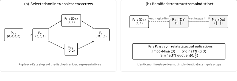
A selected confluence atlas. Solid arrows are nonlinear coalescence arrows; dashed arrows isolate degenerations of the Painlevé III leading type. The slope tuples refer to the named rank-two Lax representatives. The complete linear-system diagram also contains degenerate PV, Painlevé XXXIV, and Painlevé I nodes.

The PII rows make an important point. The Jimbo–Miwa representation has one unramified slope-$3$ point. The original Flaschka–Newell spectral system instead has a regular point and an unramified slope-$3$ point. Passing to its quadratic quotient coordinate packages the latter as the ramified pattern $(0,\tfrac32)$; the corresponding scalar apparent coordinate satisfies Painlevé XXXIV, which is nonlinearly equivalent to PII. A nonlinear Painlevé equation therefore does not determine a unique spectral singularity pattern, and a ramified quotient must not be silently identified with its covering system.

For reference, the remaining nonlinear conventions on this page are

$$\begin{aligned} \text{PIV:}\quad u'' ={}& \frac{(u')^2}{2u} + \frac32u^3 + 4Tu^2 \\ &+ 2(T^2-\alpha)u + \frac{\beta}{u}, \\ \text{PII:}\quad u'' ={}& 2u^3+Tu+\alpha. \end{aligned}$$

The atlas is a guide to formal types, not a claim that the indicated Heun equation is automatically the scalar component of every Lax pair in that row.

The three PIII strata are not interchangeable

Fix the four-parameter form

$$u'' = \frac{(u')^2}{u} - \frac{u'}{T} + \frac{\alpha u^2+\beta}{T} + \gamma u^3 + \frac{\delta}{u}.$$

The three nonquadrature strata are

Type	Coefficient stratum	Standard Lax slopes	Essential parameters
$D_6$	$\gamma\delta\ne0$	$(1,1)$	$2$
$D_7$	$\gamma=0$, $\alpha\delta\ne0$, or the reciprocal case $\delta=0$, $\beta\gamma\ne0$	$(1,\tfrac12)$	$1$
$D_8$	$\gamma=\delta=0$, $\alpha\beta\ne0$	$(\tfrac12,\tfrac12)$	$0$

The labels $D_6,D_7,D_8$ abbreviate the affine root types $D_6^{(1)}$, $D_7^{(1)}$, and $D_8^{(1)}$ of Okamoto’s spaces of initial conditions. They are not matrix sizes, pole counts, or numbers of Stokes sectors.

The parameter count follows without geometry. Under

$$T=aX, \qquad u=bU,$$

the coefficients transform as

$$\begin{aligned} (\alpha,\beta,\gamma,\delta) \longmapsto \left( ab\alpha,\, \frac{a}{b}\beta,\, a^2b^2\gamma,\, \frac{a^2}{b^2}\delta \right). \end{aligned}$$

The two nonzero scaling freedoms normalize two coefficients. On the $D_6$ stratum this leaves two continuous parameters; on $D_7$, one; and on $D_8$, none. Further vanishings can leave the Painlevé strata and enter Riccati or quadrature cases. In particular, if $\alpha=\gamma=0$ or $\beta=\delta=0$, one should not relabel the result as a generic member of the next $D$-type.

Exact D₇ seed on a fixed branch

Take

$$(\alpha,\beta,\gamma,\delta) = (8,0,0,-1)$$

and choose a branch of $T^{1/3}$ on a simply connected sector avoiding $T=0$. Then

$$u(T)=\frac12T^{1/3}$$

is an exact $P_{\mathrm{III}}(D_7)$ solution. Indeed,

$$u' = \frac16T^{-2/3}, \qquad u'' = -\frac19T^{-5/3},$$

while

$$\frac{(u')^2}{u} - \frac{u'}{T} = \frac1{18}T^{-5/3} - \frac16T^{-5/3} = -\frac19T^{-5/3},$$

and the force terms cancel:

$$\frac{8u^2}{T} - \frac1u = 2T^{-1/3} - 2T^{-1/3} =0.$$

The cube-root branch is anchored at the fixed singular point $T=0$. It therefore does not violate the Painlevé property, which excludes movable critical branching.

Regular monodromy becomes wild data

Before collision, the two local monodromies are conjugate to exponentials of the scaled residues. With residues of order $\varepsilon^{-1}$, those matrices usually oscillate or grow without a componentwise limit. The correct limiting objects are extracted only after choosing sectors, formal gauges, and connecting normalizations.

For a generic rank-two slope-$1$ irregular point, the local data consist of:

• its irregular type and associated exponential torus;
• its formal monodromy;
• an ordered pair of unipotent Stokes factors;
• links from sectorial bases to the remaining singular points.

The product of appropriately ordered cluster monodromies can converge to the full analytic monodromy around the irregular point, which combines formal monodromy with the ordered Stokes factors. It should not be identified with either Stokes factor separately. Which regular loops belong to a cluster, which sector is first, and which conjugations are removed all depend on the chosen marking.

This explains how confluence preserves a monodromy dimension even though the number of regular punctures decreases: tame conjugacy data are repackaged as formal and Stokes data. Precise convergence can depend on a controlled sequence of $\varepsilon$ values because the divergent formal exponents themselves retain a rapidly varying fractional part.

Tau functions require a finite part

The JMU differential is the safest object to confluence. Let $t=t_\varepsilon(T)$ and suppose that, after pulling back the parent family and fixing the gauge convention,

$$t_\varepsilon^* \omega_{\mathrm{JMU}}^{\mathrm{parent}} = \dd F_\varepsilon(T) + \omega_{\mathrm{JMU}}^{\mathrm{child}} + o(1).$$

Equivalently, for one deformation time,

$$t_\varepsilon'(T) H_{\mathrm{parent}} \bigl(t_\varepsilon(T)\bigr) = \partial_TF_\varepsilon(T) + H_{\mathrm{child}}(T) + o(1).$$

The finite child tau function is then

$$\tau_{\mathrm{child}}(T) = \lim_{\varepsilon\to0} C_\varepsilon \exp[-F_\varepsilon(T)] \tau_{\mathrm{parent}} \bigl(t_\varepsilon(T)\bigr),$$

when the limit exists locally uniformly and is not identically zero. Here $C_\varepsilon$ is independent of $T$, although it may depend on the scaled monodromy data.

The two normalizations have different roles:

• $\exp[-F_\varepsilon(T)]$ removes the time-dependent exact part required to match the declared child JMU differential; this includes its divergent terms and may include a finite convention-matching term;
• $C_\varepsilon$ is the ordinary time-independent ambiguity left by the definition $\dd\log\tau=\omega_{\mathrm{JMU}}$.

There is no universal counterterm $F_\varepsilon$. It depends on the confluence arrow, time coordinate, gauge, exponent lifts, and determinant-line convention. A formula that suppresses it is not convention invariant.

Because the exponential counterterm is nonzero on the chosen time cover, it does not change the finite-$\varepsilon$ zero set. Passing zeros to the limit still requires locally uniform convergence to a nonzero holomorphic limit. Hurwitz’s theorem, not formal coefficient matching, is the relevant analytic principle.

An exact commuting tau ledger

A reducible example isolates every divergent power. Let

$$D= \begin{pmatrix} 1&0\\ 0&-1 \end{pmatrix}, \qquad R= \begin{pmatrix} 2&0\\ 0&-2 \end{pmatrix},$$

and

$$C_t= \begin{pmatrix} \tfrac13&0\\ 0&-\tfrac13 \end{pmatrix}, \qquad C_1= \begin{pmatrix} \tfrac15&0\\ 0&-\tfrac15 \end{pmatrix}.$$

For

$$A_0=D, \qquad A_t=\frac{R}{\varepsilon}+C_t, \qquad A_1=-\frac{R}{\varepsilon}+C_1, \qquad t=1+\varepsilon T,$$

all residues commute, so the Schlesinger equations keep them constant. Although the exponent difference at $z=0$ is resonant, the connection is exactly diagonal; the displayed diagonal Levelt factors fix the local choice used in the pairwise trace formula. The spectral and deformation matrices have the limits

$$\begin{aligned} A_{\mathrm{lim}}(z,T) &= \frac{D}{z} + \frac{TR}{(z-1)^2} + \frac{C_t+C_1}{z-1}, \\ B_{\mathrm{lim}}(z,T) &= -\frac{R}{z-1}. \end{aligned}$$

On declared branches, an exact limiting fundamental matrix is

$$Y_{\mathrm{lim}}(z,T) = z^D (z-1)^{C_t+C_1} \exp\left[-\frac{TR}{z-1}\right].$$

The parent trace exponents are

$$\operatorname{Tr}(DA_t) = \frac4\varepsilon+\frac23$$

and

$$\operatorname{Tr}(A_tA_1) = -\frac8{\varepsilon^2} - \frac8{15\varepsilon} + \frac2{15}.$$

Consequently the four-pole JMU tau function is

$$\tau_\varepsilon(t) = C_\varepsilon\, t^{\,4/\varepsilon+2/3} (t-1)^{-8/\varepsilon^2-8/(15\varepsilon)+2/15}.$$

Choose the $\varepsilon$-dependent constant to remove the pure power of $\varepsilon$ coming from $t-1=\varepsilon T$. The remaining pullback is

$$\widehat\tau_\varepsilon(T) = (1+\varepsilon T)^{4/\varepsilon+2/3} T^{-8/\varepsilon^2-8/(15\varepsilon)+2/15}.$$

The full time-dependent exact factor required to match the standard JMU differential of the displayed child pair is removed by

$$\tau_\varepsilon^{\mathrm{ren}}(T) = T^{8/\varepsilon^2+8/(15\varepsilon)-2/15} \widehat\tau_\varepsilon(T),$$

and therefore

$$\tau_\varepsilon^{\mathrm{ren}}(T) \longrightarrow \exp(4T).$$

This agrees directly with the child JMU residue. With $w=z-1$, write

$$\widehat\Phi(w)=(1+w)^D, \qquad \Theta(w,T) = -\frac{TR}{w} + (C_t+C_1)\log w.$$

Then

$$\begin{aligned} \omega_{\mathrm{JMU}}^{\mathrm{lim}} &= -\underset{w=0}{\operatorname{res}} \operatorname{Tr} \left[ \frac{D}{1+w} \left(-\frac{R}{w}\right) \right]\dd T \\ &= \operatorname{Tr}(DR)\,\dd T = 4\,\dd T. \end{aligned}$$

Thus, in the standard child convention,

$$\partial_T\log\tau_{\mathrm{lim}} = 4.$$

Subtracting only the divergent powers would instead leave $\exp(4T)T^{2/15}$. The extra power depends on the parent split into $C_t$ and $C_1$, while the limiting connection knows only $C_t+C_1$; it is therefore not the standard JMU tau function of the displayed child pair.

This example verifies the surviving polar moment, the limiting zero-curvature pair, and both kinds of tau normalization. It has trivial Stokes matrices because it is diagonal. It is therefore a normalization benchmark, not a model of generic Painlevé V transcendents.

Heun geometry survives with qualifications

The atlas matches the true-singularity geometries introduced in the Heun confluence hierarchy:

• PVI and the general Heun equation have four regular true singularities;
• PV and confluent Heun have two regular points and one slope-$1$ irregular point;
• $P_{\mathrm{III}}(D_6)$ and double-confluent Heun have two unramified slope-$1$ points;
• PIV and biconfluent Heun have one regular and one slope-$2$ point;
• the Jimbo–Miwa PII system and triconfluent Heun have one slope-$3$ point.

This is a match of formal singularity patterns, not an identity of equations. A cyclic scalar reduction generally introduces an apparent singularity. Recovering a canonical confluent Heun equation requires an apparent-pole specialization, a scalar gauge, a coordinate choice, and an exponent and accessory dictionary. The ramified $D_7$, $D_8$, and Flaschka–Newell quotient types are not generic rows of the five-name unramified Heun hierarchy; neither is the original two-point Flaschka–Newell realization.

In particular, a confluent Heun accessory cannot be obtained by simply putting $t=1$ into the PVI–Heun formula of the preceding page. One must first confluence the matrix connection and its tau differential, then perform the scalar specialization in the limiting chart.

A practical confluence audit

Before accepting a Painlevé or Heun confluence, record all of the following:

1. the scaled spectral coordinate and deformation time;
2. every pole position, residue, exponent lift, and equation parameter;
3. the matrix gauge and any scalar Liouville gauge;
4. the limiting formal type, including ramification and slope;
5. the sectorial bases, Stokes ordering, and surviving connection links;
6. the pulled-back JMU differential and the full exact counterterm needed to match the child convention;
7. the apparent-pole condition used in a scalar reduction;
8. an independent check, such as a direct recurrence, a numerical connection matrix, or an exact reducible family.

This ledger prevents three different operations—pole collision, scalar specialization, and boundary quantization—from being compressed into one formal substitution.

Common pitfalls

Colliding positions without scaling residues. Bounded residues only add their simple-pole coefficients. A nonzero higher polar moment requires a correlated divergence of residues or exponent lifts.

Taking monodromy matrices term by term. Individual regular monodromies usually have no limit. Formal monodromy and Stokes matrices arise from sectorially normalized combinations with a declared marking.

Writing only “Painlevé III.” The $D_6$, $D_7$, and $D_8$ strata have different parameter counts and different ramification types. Additional coefficient vanishings can instead produce quadrature cases.

Assuming the tau function converges unchanged. The exact differential needed to match the child convention must be subtracted before taking the limit; it can contain both divergent and finite terms. A remaining time-independent normalization is still free.

Equating a Lax type with a named Heun equation. Matching true singularities does not remove the apparent scalar pole or fix a canonical scalar gauge and accessory parameter.

Exercises

1. Uniform control of the two-pole collision

Derive the exact error term for $A^{(\varepsilon)}-A^{(0)}$. If a compact set $K$ satisfies $|z|\geq r>0$ on $K$, prove that the convergence is uniformly $O(\varepsilon)$ for $|\varepsilon|<r/2$.

Solution

Direct subtraction gives

$$A^{(\varepsilon)}-A^{(0)} = \varepsilon \left[ \frac{R}{z^2(z-\varepsilon)} + \frac{C_1}{z(z-\varepsilon)} \right].$$

For $z\in K$ and $|\varepsilon|<r/2$, $|z-\varepsilon|\geq r/2$. In any submultiplicative matrix norm,

$$\sup_K \left\| A^{(\varepsilon)}-A^{(0)} \right\| \leq |\varepsilon| \left( \frac{2\lVert R\rVert}{r^3} + \frac{2\lVert C_1\rVert}{r^2} \right).$$

This is a uniform $O(\varepsilon)$ estimate away from the shrinking collision disk.

2. Stokes rays of the elementary irregular model

For $R=\sigma_3$, find the walls on which the two formal exponentials $\exp(\mp1/z)$ have equal magnitude.

Solution

Their ratio is $\exp(-2/z)$. Equal magnitude means

$$\operatorname{Re}\frac{2}{z}=0.$$

Writing $z=re^{\ii\vartheta}$ gives $\operatorname{Re}(2/z)=2\cos\vartheta/r$, so the walls are $\vartheta=\pi/2$ and $3\pi/2$. Whether these are called Stokes or anti-Stokes rays depends on the naming convention; the invariant statement is the equal-magnitude condition.

3. The PVI to PV force term

Substitute the parameter scaling of this page into the standard PVI equation and derive the finite $\delta_5Q(Q+1)/(Q-1)$ term.

Solution

After multiplying PVI by $\varepsilon^2$, the common potential prefactor tends to

$$\frac{Q(Q-1)^2}{T^2}.$$

The two $\delta_5$ contributions inside the braces combine as

$$\frac{\delta_5T}{\varepsilon} \left[ \frac{1+\varepsilon T} {(Q-1-\varepsilon T)^2} - \frac1{(Q-1)^2} \right].$$

For $a=Q-1$,

$$\frac{1+\varepsilon T}{(a-\varepsilon T)^2} = \frac1{a^2} + \varepsilon T \left( \frac1{a^2} + \frac2{a^3} \right) + O(\varepsilon^2).$$

The bracket therefore tends, after division by $\varepsilon$, to $T(Q+1)/(Q-1)^3$. Multiplication by the outer $T$ and by the common prefactor gives

$$\frac{Q(Q-1)^2}{T^2} \frac{\delta_5T^2(Q+1)}{(Q-1)^3} = \frac{\delta_5Q(Q+1)}{Q-1}.$$

4. Counting the PIII parameters

Derive the coefficient transformation under $T=aX$, $u=bU$ and explain the counts $2,1,0$ for $D_6,D_7,D_8$.

Solution

Since $u'=bU_X/a$ and $u''=bU_{XX}/a^2$, multiplication by $a^2/b$ restores the standard derivative terms. The force coefficients become

$$\left( ab\alpha,\, \frac{a}{b}\beta,\, a^2b^2\gamma,\, \frac{a^2}{b^2}\delta \right).$$

Two independent nonzero scalings normalize two nonzero coefficients. The $D_6$ stratum starts with four coefficients and leaves two moduli. The $D_7$ stratum starts with three and leaves one. The $D_8$ stratum starts with two and leaves none.

5. The fixed cubic-root branch

Verify the $D_7$ seed $u(T)=T^{1/3}/2$ and explain why its branch point does not contradict the Painlevé property.

Solution

The derivative and force calculations are displayed above: the derivative terms equal $-T^{-5/3}/9$, and the two force terms cancel. The only branch point is at $T=0$, a fixed singularity of the differential equation. The Painlevé property rules out movable critical branch points whose locations depend on initial data; it does not require single-valuedness around fixed singularities.

6. Renormalizing a logarithmic derivative

Assume

$$t_\varepsilon'H_{\mathrm{parent}} = \partial_TF_\varepsilon + H_{\mathrm{child}} + O(\varepsilon)$$

locally uniformly. Show that the logarithmic derivative of $\exp(-F_\varepsilon)\tau_{\mathrm{parent}}(t_\varepsilon(T))$ converges to $H_{\mathrm{child}}$.

Solution

By the chain rule and the definition of the parent tau function,

$$\begin{aligned} \partial_T\log \left[ \ee^{-F_\varepsilon(T)} \tau_{\mathrm{parent}}(t_\varepsilon(T)) \right] &= -\partial_TF_\varepsilon + t_\varepsilon'H_{\mathrm{parent}} \\ &= H_{\mathrm{child}}+O(\varepsilon). \end{aligned}$$

Integration on a simply connected time domain determines the limiting tau function up to a $T$-independent factor. Convergence of logarithmic derivatives alone does not fix that factor or prove convergence across zeros.

7. Related PII spectral types

Why can PII have the Jimbo–Miwa pattern $(3)$ and the original Flaschka–Newell pattern $(0,3)$, while a related ramified quotient has pattern $(0,\tfrac32)$?

Solution

A Painlevé equation is the nonlinear compatibility condition of a Lax pair, but the Lax representation is not unique. The Jimbo–Miwa and original Flaschka–Newell pairs use different spectral connections and are not related by a harmless rational gauge preserving the same formal type. The quadratic quotient of the latter halves its slope $3$ to the ramified slope $3/2$ and naturally yields Painlevé XXXIV, whose dependent variable is nonlinearly related to a PII solution. Cover, quotient, and nonlinear equivalence are different operations.

8. From a Lax collision to a confluent Heun accessory

List the additional data needed before the accessory of a scalar confluent Heun equation can be called the confluence of the page-5 Heun accessory.

Solution

One must specify the scaled spectral coordinate and time, the matrix gauge, the diverging exponent lifts, the cyclic vector used in scalar reduction, the apparent-pole specialization, the scalar gauge to the chosen confluent Heun convention, the limiting accessory dictionary, and the time-dependent tau counterterm. A boundary or spectral interpretation additionally requires the relevant sectorial bases and monodromy or Stokes constraints.

References

• M. Jimbo, T. Miwa, and K. Ueno, “Monodromy Preserving Deformation of Linear Ordinary Differential Equations with Rational Coefficients. I”, Physica D 2 (1981), 306–352. General irregular deformation theory, generalized monodromy data, and the JMU tau function.
• M. Jimbo and T. Miwa, “Monodromy Preserving Deformation of Linear Ordinary Differential Equations with Rational Coefficients. II”, Physica D 2 (1981), 407–448. Classical Painlevé Lax pairs, Hamiltonians, and degeneration formulae.
• P. A. Clarkson, “Painlevé Transcendents: Differential Equations,” DLMF §32.2. Standard nonlinear equation conventions and coalescence scalings.
• Y. Ohyama and S. Okumura, “A Coalescent Diagram of the Painlevé Equations from the Viewpoint of Isomonodromic Deformations”, Journal of Physics A 39 (2006), 12129–12151. The complete rank-two linear-system diagram, ramified types, and distinct PII realizations.
• M. van der Put and M.-H. Saito, “Moduli Spaces for Linear Differential Equations and the Painlevé Equations”, Annales de l’Institut Fourier 59 (2009), 2611–2667. Katz invariants, wild monodromy spaces, and the ten rank-two families.
• M. Klimeš, “Wild Monodromy of the Fifth Painlevé Equation and Its Action on Wild Character Varieties: An Approach of Confluence”, Annales de l’Institut Fourier 74 (2024), 121–192. Precise PVI to PV confluence on the Lax and wild-character-variety sides.
• R. J. Buckingham and P. D. Miller, “On the Algebraic Solutions of the Painlevé-III (D₇) Equation”, Physica D 441 (2022), 133493. Algebraic $D_7$ solutions and their Riemann–Hilbert realization.
• O. Lisovyy, H. Nagoya, and J. Roussillon, “Irregular Conformal Blocks and Connection Formulae for Painlevé V Functions”, Journal of Mathematical Physics 59 (2018), 091409. A concrete tau-function realization obtained through PVI to PV confluence.
• K. Iwasaki, H. Kimura, S. Shimomura, and M. Yoshida, From Gauss to Painlevé: A Modern Theory of Special Functions, Vieweg, 1991. Systematic background on confluence, monodromy-preserving deformation, and Painlevé geometry.