Horizon, Boundary, and Angular Canonical Bases

Separation and singularity classification produce a two-dimensional solution space at each fixed $(\omega,A)$. They do not identify which one-dimensional line is smooth on a future horizon, radiative at infinity, admissible at a timelike AdS boundary, or regular at an angular axis. Those lines are the local inputs to the global connection problem.

This page constructs them in the Fourier convention $\ee^{-\ii\omega t+\ii m\phi}$. The scalar Kerr equation supplies the main laboratory; Schwarzschild–de Sitter fixes the cosmological-horizon signs; Fefferman–Graham coordinates fix the AdS weights; and the spin-$s$ angular equation supplies the axis bases. Every word such as “ingoing,” “outgoing,” or “canonical” will be tied to a coordinate, a branch, a leading coefficient, and—at an irregular endpoint—a sector or continuation prescription.

The output is a collection of normalized local lines, not yet a spectrum. The next page will compare endpoint lines by Wronskians and recurrence minimality. The later holography page will add counterterms and turn AdS coefficients into normalized retarded observables.

First reading

Follow future event horizon → flat infinity → Abel check → cosmological horizon → AdS boundary → angular axes. The real-frequency flux calculation, resonant strata, spin-$s$ weights, and extremal sectorial basis may wait for a second pass.

Status ledger

Construction	Status and scope
Subextremal scalar Kerr horizon pair	Exact in the displayed Boyer–Lindquist and Fourier convention
Asymptotically flat Jost pair	Sectorial for $\omega\ne0$; the causal analytic continuation is part of the definition
Same-endpoint Abel Wronskians	Exact normalization checks for the scalar equation
Radial flux and superradiant sign	Exact only on the real-frequency, real-accessory slice
Schwarzschild–de Sitter outer pair	Exact sign calibration in the static patch
AdS slow and fast scalar pair	Exact leading nonresonant asymptotics; admissibility depends on the theory and quantization
Spin-$s$ angular pole lines	Exact in the displayed spin-frame convention
Extremal Kerr horizon pair	Formal sectorial asymptotics away from the synchronous frequency
Cross-endpoint alignment or QNM equation	Deferred to the next page
Renormalized retarded correlator	Deferred to the holographic-correlator page

A canonical line needs a passport

Reuse the scalar Kerr equation from the separation page:

$$\frac{\dd}{\dd r} \left( \Delta R' \right) + \left( \frac{K^2}{\Delta}-\lambda \right)R =0,$$

with

$$\begin{aligned} \Delta&=(r-r_+)(r-r_-), &K(r)&=\omega(r^2+a^2)-am,\\ \lambda&=A+a^2\omega^2-2am\omega, &r_\pm&=M\pm\sqrt{M^2-a^2}. \end{aligned}$$

Unless a subsection says otherwise, assume $M>0$, $|a|<M$, and a neutral massless scalar. The ordered Wronskian convention is

$$\Wr[f,g]=fg'-f'g.$$

A reproducible endpoint vector requires more than its leading exponential:

Passport entry	Required datum
Operator	Exact radial or angular unknown and accessory convention
Local geometry	Endpoint, local coordinate, and orientation of the physical interval
Branch	A branch of every $\operatorname{Log}$ used in complex powers
Ordering	Which vector is first and which is second
Normalization	Leading coefficient, or an equivalent same-endpoint Wronskian
Irregular endpoint	Stokes sector and lateral or analytic-continuation prescription
Exceptional stratum	Frequencies or masses at which exponents collide or the rank changes

Three levels should be kept distinct. A formal pair is an ordered pair of formal Frobenius or exponential series. A normalized analytic basis is a pair of actual solutions obtained after branches and sectors have been fixed. A physical line is the span of one basis vector selected by future regularity, radiation, or boundary admissibility. Rescaling a vector changes connection coefficients, while its line is unchanged.

The future event horizon selects a geometric line

Set

$$x=r-r_+, \qquad \Omega_+=\frac{a}{r_+^2+a^2}, \qquad \widetilde\omega_+=\omega-m\Omega_+,$$

and use the positive outer-horizon surface gravity

$$\kappa_+ = \frac{r_+-r_-}{2(r_+^2+a^2)}.$$

The tortoise coordinate is determined up to an additive constant by

$$\frac{\dd r_*}{\dd r} = \frac{r^2+a^2}{\Delta}.$$

On a chosen branch of $\operatorname{Log}(x/r_0)$,

$$r_* = \frac{1}{2\kappa_+} \operatorname{Log}\!\left(\frac{x}{r_0}\right) +O(1), \qquad x\to0,$$

where $r_0>0$ and the finite part fix the otherwise arbitrary additive constant. The indicial roots give the normalized pair

$$\begin{aligned} R_H^{\mathrm{in}} &= \left(\frac{x}{r_0}\right)^{-\ii\widetilde\omega_+/(2\kappa_+)} \left(1+O(x)\right),\\ R_H^{\mathrm{out}} &= \left(\frac{x}{r_0}\right)^{+\ii\widetilde\omega_+/(2\kappa_+)} \left(1+O(x)\right). \end{aligned}$$

After a compatible choice of the finite part of $r_*$, these phases are

$$R_H^{\mathrm{in/out}} \sim \ee^{\mp\ii\widetilde\omega_+r_*}.$$

The labels are geometric, not mnemonic. Introduce future-ingoing Kerr coordinates

$$v=t+r_*, \qquad \widetilde\phi = \phi+ \int^r\frac{a}{\Delta(\rho)}\,\dd\rho.$$

Near $r_+$,

$$\widetilde\phi = \phi+\Omega_+r_*+O(1).$$

The full separated field built from $R_H^{\mathrm{in}}$ therefore has the form

$$\begin{aligned} &\ee^{-\ii\omega t+\ii m\phi} R_H^{\mathrm{in}} \\ &\qquad\sim \ee^{-\ii\omega v+\ii m\widetilde\phi} \times \left( \text{smooth nonzero factor} \right). \end{aligned}$$

It extends through the future event horizon. The other line is naturally regular across the past horizon instead. This argument also explains the co-rotating frequency $\widetilde\omega_+$: horizon generators see $\partial_t+\Omega_+\partial_\phi$, not $\partial_t$ alone.

For Schwarzschild, $a=0$, $r_+=2M$, and $\kappa_+=1/(4M)$. Choosing $r_0=2M$ gives

$$R_H^{\mathrm{in/out}} \sim \left(\frac{r-2M}{2M}\right)^{\mp2\ii M\omega}.$$

With $z=r/(2M)$ and $\Omega=2M\omega$, the future-ingoing factor is $(z-1)^{-\ii\Omega}$. This is exactly the factor used in the preceding page’s Schwarzschild-to-confluent-Heun crosswalk.

Coalescing horizon labels

At $\widetilde\omega_+=0$, the two indicial roots coincide. One scalar solution is analytic and a reduction-of-order companion contains $\operatorname{Log}(x/r_0)$. The words ingoing and outgoing no longer distinguish two Frobenius lines. More generally, an integral exponent difference permits a logarithmic resonance and requires a declared limiting or Levelt normalization.

Expert extension: the Teukolsky radial weights

The algebraic prefactors depend on the master variable. For the Kinnersley-frame spin-$s$ Teukolsky radial function in a standard convention,

$$R_{s,H}^{\mathrm{in}} \sim \Delta^{-s} \ee^{-\ii\widetilde\omega_+r_*}, \qquad R_{s,H}^{\mathrm{out}} \sim \ee^{+\ii\widetilde\omega_+r_*}.$$

At flat infinity the corresponding leading weights are

$$R_{s,\infty}^{\mathrm{out}} \sim r^{-2s-1}\ee^{+\ii\omega r_*}, \qquad R_{s,\infty}^{\mathrm{in}} \sim r^{-1}\ee^{-\ii\omega r_*}.$$

These are not contradictions with the scalar formulas: changing tetrad or master variable changes powers and Wronskian weights. A passport must name the variable before borrowing an endpoint formula.

Flat infinity is a sectorial Jost problem

For the scalar Kerr equation,

$$r_* = r+2M\operatorname{Log}\!\left(\frac r{r_0}\right) +O(r^{-1}), \qquad r\to\infty.$$

When $\omega\ne0$, infinity is rank-one irregular. Choose a branch of $\operatorname{Log}r$, an angular lift of a Stokes sector, and unit leading coefficients. The formal radiation pair is

$$\begin{aligned} R_\infty^{\mathrm{out}} &= \frac1r\ee^{+\ii\omega r_*} \left(1+O(r^{-1})\right),\\ R_\infty^{\mathrm{in}} &= \frac1r\ee^{-\ii\omega r_*} \left(1+O(r^{-1})\right). \end{aligned}$$

Equivalently,

$$\begin{aligned} R_\infty^{\mathrm{out}} &= \frac{\ee^{+\ii\omega r}}r \left(\frac r{r_0}\right)^{+2\ii M\omega} \left(1+O(r^{-1})\right),\\ R_\infty^{\mathrm{in}} &= \frac{\ee^{-\ii\omega r}}r \left(\frac r{r_0}\right)^{-2\ii M\omega} \left(1+O(r^{-1})\right), \end{aligned}$$

where the dimensionless powers inherit the same scale and logarithm branch as $r_*$. The full outgoing field depends on retarded time $u=t-r_*$; the incoming field depends on advanced time $v=t+r_*$. “Outgoing” is therefore a causal phase label, not a synonym for spatial decay.

The ratio of the two exponential parts is $\ee^{2\ii\omega r}$. Their equal-magnitude rays obey

$$\operatorname{Re}(2\ii\omega r)=0.$$

Within a suitable open sector, summation or a Jost integral equation turns each formal series into an analytic solution. Crossing an equal-magnitude ray reverses dominance. A Stokes jump is instead tied to a separately declared singular or lateral direction; a nonzero multiplier is additional analytic data. Thus a leading exponential by itself does not globally define a vector. This book states the phase condition because sources interchange the names “Stokes” and “anti-Stokes” for related rays.

The causal continuation fixes the radiation line

With $\ee^{-\ii\omega t}$, a retarded transform is initially analytic for sufficiently large $\operatorname{Im}\omega>0$. In that half-plane, $R_H^{\mathrm{in}}$ decays as $r_*\to-\infty$ and $R_\infty^{\mathrm{out}}$ decays as $r_*\to+\infty$. They can be selected by convergent endpoint constructions and then analytically continued in $\omega$.

This continuation matters in the lower half-plane. A damped resonance has $\operatorname{Im}\omega<0$, so its outgoing radial factor grows on the positive real $r$ axis. Moreover, a dominant asymptotic expansion alone may not exclude an exponentially subdominant admixture. The physical outgoing line is the continuation of the causal Jost line, not “whichever solution decays at the QNM frequency.”

The shift $r_*\mapsto r_*+C$ rescales $R_\infty^{\mathrm{out/in}}$ by $\ee^{\pm\ii\omega C}$. It changes normalized vectors and connection coefficients but not their spans. The scale $r_0$ and additive constant therefore belong in any comparison of amplitudes.

At $\omega=0$, the exponential parts disappear and infinity is no longer the same irregular endpoint. For a scalar multipole the static branches behave as $r^\ell$ and $r^{-\ell-1}$; wave labels must be replaced by a new static basis. The zero-frequency degeneration is also tied to the branch structure responsible for asymptotically flat late-time tails.

Weighted Wronskians audit both endpoint pairs

Abel’s identity applied directly to the scalar radial equation gives

$$\mathcal W[R_1,R_2] = \Delta\Wr[R_1,R_2], \qquad \frac{\dd\mathcal W}{\dd r}=0.$$

The unit-leading ordered pairs

$$\left( R_H^{\mathrm{in}},R_H^{\mathrm{out}} \right), \qquad \left( R_\infty^{\mathrm{in}},R_\infty^{\mathrm{out}} \right)$$

obey the exact same-endpoint checks

$$\begin{aligned} \mathcal W \left[ R_H^{\mathrm{in}},R_H^{\mathrm{out}} \right] &=2\ii K(r_+),\\ \mathcal W \left[ R_\infty^{\mathrm{in}},R_\infty^{\mathrm{out}} \right] &=2\ii\omega. \end{aligned}$$

For the first identity, use $\Delta\sim(r_+-r_-)x$ and the difference of the two horizon exponents. For the second, use $\Delta\sim r^2$ and $\dd r_*/\dd r\to1$. Each identity checks the basis order, exponent signs, and leading normalization at once. They are bilinear statements and remain valid for complex $\omega$.

Expert check: real-frequency flux and superradiance

When $\omega$, $A$, and the background parameters are real, complex conjugation preserves the scalar radial equation. Then

$$J_r[R] = \frac{\Delta}{2\ii} \left( R^*R'-RR'^* \right)$$

is constant. For the unit-leading endpoint vectors,

$$\begin{aligned} J_r\!\left[R_H^{\mathrm{out/in}}\right] &= \pm(r_+^2+a^2)\widetilde\omega_+,\\ J_r\!\left[R_\infty^{\mathrm{out/in}}\right] &= \pm\omega. \end{aligned}$$

Suppose a real-frequency scattering solution is future-ingoing at the horizon and has

$$\begin{aligned} R&\sim A_{\mathrm{in}}R_\infty^{\mathrm{in}} +A_{\mathrm{out}}R_\infty^{\mathrm{out}},\\ R&\sim B_{\mathrm{in}}R_H^{\mathrm{in}}. \end{aligned}$$

Flux conservation yields

$$\begin{aligned} \omega \left( |A_{\mathrm{in}}|^2-|A_{\mathrm{out}}|^2 \right) ={}& (r_+^2+a^2)\widetilde\omega_+ |B_{\mathrm{in}}|^2. \end{aligned}$$

For $\omega>0$ and $\widetilde\omega_+<0$, the reflected amplitude exceeds the incident amplitude: the horizon-ingoing line carries negative $t$-energy and the wave is superradiantly amplified. The word “ingoing” has not changed meaning; the energy sign has.

For complex $\omega$, $R^*$ solves an equation at $\omega^*$ rather than at $\omega$. The conjugate current is then not a conserved analytic spectral test. Use the bilinear Abel Wronskian instead.

A cosmological horizon reverses the tortoise orientation

Schwarzschild–de Sitter is the cleanest sign calibration. In the static region $r_b<r<r_c$, let

$$f(r)=1-\frac{2M}{r}-\frac{\Lambda r^2}{3}, \qquad \frac{\dd r_*}{\dd r}=\frac1{f(r)},$$

where $r_b$ is the black-hole event horizon and $r_c$ the cosmological horizon. Define positive surface-gravity magnitudes and inward distances by

$$\begin{aligned} \kappa_b&=\frac12f'(r_b)>0, &x_b&=r-r_b,\\ \kappa_c&=-\frac12f'(r_c)>0, &x_c&=r_c-r. \end{aligned}$$

Choose positive reference lengths $\ell_b$ and $\ell_c$ for the two local logarithms. Then

$$r_* = \frac{1}{2\kappa_b} \operatorname{Log}\!\left(\frac{x_b}{\ell_b}\right) - \frac{1}{2\kappa_c} \operatorname{Log}\!\left(\frac{x_c}{\ell_c}\right) +O(1).$$

Consequently, $r_*\to-\infty$ at the event horizon but $r_*\to+\infty$ at the cosmological horizon. The two future-selected lines are

$$\begin{aligned} R_b^{\mathrm{in}} &= \left(\frac{x_b}{\ell_b}\right)^{-\ii\omega/(2\kappa_b)} \left(1+O(x_b)\right) \sim\ee^{-\ii\omega r_*},\\ R_c^{\mathrm{out}} &= \left(\frac{x_c}{\ell_c}\right)^{-\ii\omega/(2\kappa_c)} \left(1+O(x_c)\right) \sim\ee^{+\ii\omega r_*}. \end{aligned}$$

The first depends on advanced time $v=t+r_*$ and crosses the future event horizon. The second depends on retarded time $u=t-r_*$ and crosses the future cosmological horizon outward from the static patch. Notice that the same negative power of the positive endpoint distance corresponds to opposite signs of the tortoise phase.

For a rotating or charged horizon the invariant local frequency is replaced schematically by

$$\widetilde\omega_h = \omega-m\Omega_h-q\Phi_h.$$

This formula is safe only after the time, azimuthal, electromagnetic-gauge, and horizon-generator conventions have been frozen. In Kerr–de Sitter or Kerr–AdS, a rotating-boundary frame and a nonrotating-boundary frame assign different printed values to $\omega$ and $\Omega_h$ while preserving the coherent combination. The ratio $\widetilde\omega_h/(2\kappa_h)$ must be formed in one frame.

The AdS boundary carries slow and fast Frobenius lines

At a timelike asymptotically AdS boundary, “outgoing” is not the relevant local classification. Use a Fefferman–Graham coordinate $z\to0$ for an asymptotically $\mathrm{AdS}_{d+1}$ metric. For

$$(\Box-m_{\mathrm{eff}}^2)\Phi=0, \qquad m_{\mathrm{eff}}^2 = \mu_{\mathrm f}^2+\xi R_{\mathrm{AdS}},$$

with

$$R_{\mathrm{AdS}} = -\frac{d(d+1)}{L^2},$$

the leading radial equation is

$$z^2B''-(d-1)zB' -m_{\mathrm{eff}}^2L^2B=0.$$

Its indicial equation and roots are

$$\Delta(\Delta-d)=m_{\mathrm{eff}}^2L^2, \qquad \Delta_\pm=\frac d2\pm\nu,$$

where

$$\nu = \sqrt{ \frac{d^2}{4}+m_{\mathrm{eff}}^2L^2 }.$$

For real $\nu>0$ away from resonance, normalize the slow and fast lines by

$$\begin{aligned} B_-(z)&=z^{\Delta_-}\left(1+\cdots\right),\\ B_+(z)&=z^{\Delta_+}\left(1+\cdots\right). \end{aligned}$$

The endpoint normalization has the exact leading check

$$z^{1-d} \Wr[B_-,B_+] = 2\nu+o(1).$$

For a separated solution

$$B=\alpha B_-+\beta B_+,$$

standard quantization calls $\alpha$ the source coefficient and selects the fast line when the source is set to zero. In the alternate-quantization window

$$0<\nu<1,$$

the roles may be interchanged, subject to the theory’s stability and unitarity conditions, and an appropriate real Robin or mixed relation can define another flux-free boundary line. Its positivity is an additional global condition. The endpoint $\nu=1$ is resonant and should not be silently included. In a resonant holographic problem, the boundary relation lives in renormalized phase space—not necessarily between the raw coefficients printed above.

The two-solution boundary symplectic pairing is proportional to

$$2\nu \left( \alpha_1\beta_2-\alpha_2\beta_1 \right).$$

This explains why Dirichlet-, Neumann-, or suitable real Robin-type lines can eliminate boundary flux. It does not by itself prove stability, and it does not normalize a dual field-theory operator. The on-shell action, counterterms, finite scheme choices, and contact terms enter only on the later correlator page.

The BF point and resonant logarithms

The Breitenlohner–Freedman bound is

$$m_{\mathrm{eff}}^2L^2\ge-\frac{d^2}{4}.$$

At equality, $\nu=0$ and the roots coalesce. A normalized local pair is

$$\begin{aligned} B_0(z)&=z^{d/2}\left(1+\cdots\right),\\ B_{\log}(z)&= z^{d/2} \operatorname{Log}\!\left(\frac zL\right) \left(1+\cdots\right) +\cdots. \end{aligned}$$

Below the BF bound, $\nu$ is imaginary and the ordinary stable slow/fast passport fails. If $2\nu\in\mathbb Z$, Frobenius resonance is possible. In the usual even Fefferman–Graham scalar recursion, an actual local obstruction produces a $z^{\Delta_+}\operatorname{Log}z$ term when $\nu\in\mathbb Z_{\ge0}$. An integral exponent gap permits a logarithm; it does not prove that its coefficient is nonzero. When a log is present, the free fast coefficient changes under the scale in $\operatorname{Log}(z/L)$ and cannot by itself be a scheme-independent response.

For orientation, in $\mathrm{AdS}_4$,

$$\nu = \sqrt{ \frac94+\mu_{\mathrm f}^2L^2-12\xi }.$$

A minimally coupled massless scalar has $(\Delta_-,\Delta_+)=(0,3)$, while a conformally coupled massless scalar has $(1,2)$.

Angular axes select smooth spin-weighted lines

On a first pass, set $s=0$. Then $\lambda_0=A$, the equation below is precisely the scalar angular equation from the separation page, and both smooth pole powers reduce to $|m|$.

Let $c=a\omega$ and use the preceding page’s convention

$$\begin{aligned} -\frac1{\sin\theta} \frac{\dd}{\dd\theta} \left( \sin\theta\,S_s' \right) &+ \left[ \frac{(m+s\cos\theta)^2}{\sin^2\theta} -c^2\cos^2\theta \right. \\ &\left. \qquad +2cs\cos\theta \right]S_s = \lambda_sS_s. \end{aligned}$$

With $x=\cos\theta$, the indicial exponents at the north and south poles are

$$\begin{array}{c|c|c} \text{endpoint}&\text{local distance}&\text{exponents}\\ \hline x=1&1-x&\pm|m+s|/2\\ x=-1&1+x&\pm|m-s|/2 \end{array}$$

in this $\ee^{+\ii m\phi}$ and spin-frame convention. Normalize the smooth pole lines by

$$\begin{aligned} S_N^{\mathrm{reg}} &= (1-x)^{|m+s|/2} \left[1+O(1-x)\right],\\ S_S^{\mathrm{reg}} &= (1+x)^{|m-s|/2} \left[1+O(1+x)\right]. \end{aligned}$$

Equivalently, their leading powers in $\theta$ and $\vartheta=\pi-\theta$ are $|m+s|$ and $|m-s|$. For a scalar, both reduce to $|m|$. The negative powers give singular companions; when $m+s=0$ at the north pole or $m-s=0$ at the south pole, the repeated-root companion is logarithmic.

Smoothness here means smoothness of the complete spin-weighted section, not merely boundedness of $S_s$ in a singular spin frame. Sources with the opposite azimuthal or spin-frame convention can interchange the printed $m\pm s$ combinations. Globally admissible spin-weighted modes have $m+s,m-s\in\mathbb Z$ in this convention.

For real $c$ and real $\lambda_s$, complex conjugation preserves the displayed ODE and the current

$$J_\theta = \frac{\sin\theta}{2\ii} \left( S_s^*S_s'-S_sS_s'^* \right)$$

is conserved. In particular, on the self-adjoint two-pole spectrum, $\lambda_s$ is real and the regular eigenfunction has zero endpoint flux. At $c=0$, regularity at both poles gives

$$\lambda_s(0)=\ell(\ell+1)-s^2.$$

For complex $c$, a local leading-coefficient normalization remains useful even though the Hermitian normalization does not. The angular eigenvalue is then carried as an analytic sheet obtained by continuation from a declared seed, with possible isolated branch points. Comparing the north and south lines and solving for that sheet is a global step reserved for the next page.

Extremality replaces powers by inverse exponentials

The nonextremal formula contains $1/\kappa_+$ and cannot be specialized by setting $\kappa_+=0$. At extremal Kerr, put

$$a=M, \qquad x=r-M, \qquad \Omega_H=\frac1{2M}.$$

The scalar radial equation contains

$$K(x) = k_0+2M\omega x+\omega x^2, \qquad k_0=2M^2(\omega-m\Omega_H).$$

For $k_0\ne0$, dominant balance with $R=\exp(\beta/x)(x/r_0)^\alpha(1+O(x))$ gives

$$\beta=\pm\ii k_0, \qquad \alpha=\mp2\ii M\omega.$$

Thus a conventional ordered formal pair is

$$\begin{aligned} R_{H,\mathrm{ext}}^{\mathrm{in}} &\sim \left(\frac{x}{r_0}\right)^{-2\ii M\omega} \exp\!\left( \frac{\ii k_0}{x} \right),\\ R_{H,\mathrm{ext}}^{\mathrm{out}} &\sim \left(\frac{x}{r_0}\right)^{+2\ii M\omega} \exp\!\left( -\frac{\ii k_0}{x} \right). \end{aligned}$$

The labels can again be checked geometrically. In extremal ingoing Kerr coordinates,

$$\begin{aligned} r_* &= -\frac{2M^2}{x} +2M\operatorname{Log}\!\left(\frac{x}{r_0}\right) +x+C_*,\\ \widetilde\phi-\phi &= -\frac Mx+C_\phi. \end{aligned}$$

Because $k_0=2M^2\omega-mM$, the singular factors cancel in

$$\begin{aligned} &\ee^{+\ii\omega r_* -\ii m(\widetilde\phi-\phi)} R_{H,\mathrm{ext}}^{\mathrm{in}} \\ &\qquad= \left( \text{fixed nonzero factor} \right) \ee^{\ii\omega x} \left(1+O(x)\right). \end{aligned}$$

Thus the full field is smooth in $(v,\widetilde\phi)$ at the future extremal horizon in an admissible sector; the companion is adapted to the past horizon. These remain sectorial bases at an irregular point. Their equal-magnitude rays satisfy

$$\operatorname{Re}\!\left( \frac{2\ii k_0}{x} \right)=0.$$

The physical vectors require a specified sector and analytic continuation, not just the two formal expressions. At synchrony $k_0=0$, the inverse exponentials disappear and the horizon demotes to a regular singular point; the specialized indicial equation must be solved anew. A near-horizon scaling produces a different ODE and does not define the basis of the unscaled global extremal problem.

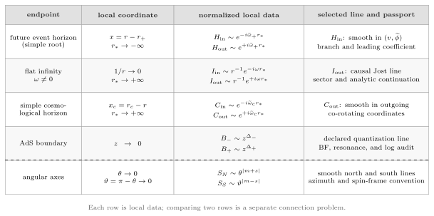
Each row is a separate endpoint passport. The selected object is a local line after its coordinate, branch, leading coefficient, and—where necessary—sector have been declared. No arrow joins two rows: their global alignment is the connection problem, not part of a local basis definition.

The endpoint certificate carried into the connection problem

Before comparing two local lines, attach a six-item certificate:

1. a positive endpoint distance and the orientation of the physical interval;
2. a horizon chart that proves any future or past regularity label;
3. logarithm branches, basis order, and leading coefficients;
4. at an irregular point, a sector and causal or lateral continuation;
5. a same-endpoint Abel Wronskian normalization check;
6. a fresh construction on zero-frequency, synchronous, resonant, BF, or extremal strata.

That compact certificate is what turns a phrase such as “ingoing Heun solution” into data that the next page can compare globally.

Common pitfalls

Choosing a mode by spatial decay. Future regularity and radiation are defined by causal coordinates and analytic continuation. Damped QNM radial functions generally grow at their open endpoints on the real spatial ray.

Using a real-frequency current at complex frequency. Complex conjugation changes $\omega$ to $\omega^*$, so the conjugate solution usually belongs to a different ODE. The bilinear Abel Wronskian is the analytic normalization check.

Importing powers without the master variable. A physical scalar, Regge–Wheeler variable, and Kinnersley-frame Teukolsky scalar have different algebraic weights. Record the dependent-variable gauge before comparing amplitudes.

Taking exceptional limits inside generic bases. At $\omega=0$, $\widetilde\omega_h=0$, $\nu=0$, or extremality, exponents or ranks collide. Return to the specialized operator and redo the local analysis.

Exercises

1. Calibrate the Schwarzschild future horizon

For the massless scalar radial equation, derive the two exponents at $r=2M$ and show directly which full separated mode is smooth in ingoing Eddington–Finkelstein time.

Solution

Set $x=r-2M$. Since $f=x/(2M)+O(x^2)$, the leading radial equation is

$$R''+\frac1xR' +\frac{4M^2\omega^2}{x^2}R=0.$$

Its roots are $\rho=\pm2\ii M\omega$. Also $r_*=2M\operatorname{Log}(x/(2M))+O(1)$, so the negative root is $R^{\mathrm{in}}\sim(x/(2M))^{-2\ii M\omega} \sim\ee^{-\ii\omega r_*}$. Multiplying by $\ee^{-\ii\omega t}$ gives $\ee^{-\ii\omega v}$ with $v=t+r_*$, which is smooth on the future horizon. The positive root depends on $t-r_*$ and is adapted to the past horizon.

2. Recover the Kerr co-rotating frequency

Derive the logarithmic parts of $r_*$ and $\widetilde\phi$ at $r_+$ and show why the regular phase contains $\omega-m\Omega_+$.

Solution

Near $r_+$,

$$\Delta=(r_+-r_-)x+O(x^2).$$

Therefore

$$\begin{aligned} r_*&= \frac{r_+^2+a^2}{r_+-r_-} \operatorname{Log}\!\left(\frac{x}{r_0}\right)+O(1),\\ \widetilde\phi-\phi&= \frac{a}{r_+-r_-} \operatorname{Log}\!\left(\frac{x}{r_0}\right)+O(1) =\Omega_+r_*+O(1). \end{aligned}$$

Consequently,

$$\ee^{-\ii\omega(t+r_*)+ \ii m(\phi+\Omega_+r_*)} = \ee^{-\ii\omega t+\ii m\phi} \ee^{-\ii(\omega-m\Omega_+)r_*}.$$

The last factor is precisely the future-ingoing radial phase.

3. Derive the same-endpoint Wronskians

Using the ordered bases on this page, derive the constants $2\ii K(r_+)$ and $2\ii\omega$.

Solution

At the horizon, write $R_H^{\mathrm{in/out}}=(x/r_0)^{\rho_{\mp}}(1+O(x))$ with

$$\rho_+-\rho_- = \frac{2\ii K(r_+)}{r_+-r_-}.$$

Then

$$\Delta\Wr \left[ R_H^{\mathrm{in}},R_H^{\mathrm{out}} \right] \longrightarrow (r_+-r_-)(\rho_+-\rho_-) =2\ii K(r_+).$$

At infinity, derivatives of the $1/r$ amplitudes cancel at leading order, while differentiating the phases gives

$$\Wr \left[ R_\infty^{\mathrm{in}},R_\infty^{\mathrm{out}} \right] = \frac{2\ii\omega}{r^2} \frac{\dd r_*}{\dd r} +O(r^{-3}).$$

Multiplication by $\Delta$ gives $2\ii\omega$. Abel’s identity makes both limits exact constants.

4. Diagnose superradiant amplification

Derive the real-frequency flux balance and determine when $|A_{\mathrm{out}}|>|A_{\mathrm{in}}|$.

Solution

For real spectral data, cross terms between oppositely directed unit Jost waves cancel in the conserved current. Hence

$$J_\infty = \omega \left( |A_{\mathrm{out}}|^2-|A_{\mathrm{in}}|^2 \right),$$

whereas a future-ingoing horizon wave gives

$$J_H = -(r_+^2+a^2)\widetilde\omega_+ |B_{\mathrm{in}}|^2.$$

Equating them yields the balance in the text. For $\omega>0$, $\widetilde\omega_+<0$ makes the right-hand side of

$$\omega \left( |A_{\mathrm{in}}|^2-|A_{\mathrm{out}}|^2 \right) = (r_+^2+a^2)\widetilde\omega_+ |B_{\mathrm{in}}|^2$$

negative, so the reflected amplitude is larger. This is the superradiant band $0<\omega<m\Omega_+$ for $m\Omega_+>0$.

5. Locate infinity equal-magnitude rays and audit a tortoise shift

Find the equal-magnitude rays of the flat-infinity pair. Then compute the effect of $r_*\mapsto r_*+C$ on the two normalized vectors and their Wronskian.

Solution

The ratio of the exponential parts is $\ee^{2\ii\omega r}$. Equal magnitude means

$$\operatorname{Re}(2\ii\omega r)=0.$$

If $r=|r|\ee^{\ii\theta}$ and $\omega=|\omega|\ee^{\ii\varphi}$, the rays satisfy

$$\theta+\varphi\in\pi\mathbb Z.$$

The tortoise shift multiplies the ordered incoming and outgoing vectors by $\ee^{-\ii\omega C}$ and $\ee^{+\ii\omega C}$. Their product is one, so $\Delta\Wr[R_\infty^{\mathrm{in}},R_\infty^{\mathrm{out}}]$ remains $2\ii\omega$, although individual connection coefficients change by the corresponding phases.

6. Fix the two Schwarzschild–de Sitter signs

Derive the event- and cosmological-horizon powers using the positive distances $x_b=r-r_b$ and $x_c=r_c-r$. Identify the future-regular null coordinate at each end.

Solution

Near $r_b$, $f=2\kappa_bx_b+O(x_b^2)$, while near $r_c$, $f=2\kappa_cx_c+O(x_c^2)$. Since $\dd x_c/\dd r=-1$,

$$r_* = \frac{1}{2\kappa_b} \operatorname{Log}\!\left(\frac{x_b}{\ell_b}\right) - \frac{1}{2\kappa_c} \operatorname{Log}\!\left(\frac{x_c}{\ell_c}\right) +O(1).$$

Thus $(x_b/\ell_b)^{-\ii\omega/(2\kappa_b)}$ is $\ee^{-\ii\omega r_*}$ and combines with the time factor into $\ee^{-\ii\omega(t+r_*)}=\ee^{-\ii\omega v}$. At the cosmological end, $(x_c/\ell_c)^{-\ii\omega/(2\kappa_c)}$ is $\ee^{+\ii\omega r_*}$ and gives $\ee^{-\ii\omega(t-r_*)}=\ee^{-\ii\omega u}$. These are the future event horizon ingoing and future cosmological-horizon outgoing lines.

7. Derive the spin-weighted pole exponents

Perform dominant balance at $\theta=0$ and $\vartheta=\pi-\theta=0$. Explain the logarithmic exceptions.

Solution

At the north pole, $\sin\theta\sim\theta$ and $\cos\theta\sim1$, so the singular part is

$$-S''-\frac1\theta S' +\frac{(m+s)^2}{\theta^2}S=0.$$

For $S\sim\theta^\rho$, the indicial equation is $\rho^2=(m+s)^2$, giving $\rho=\pm|m+s|$. At the south pole, $\cos\theta\sim-1$ and the same calculation in $\vartheta$ gives $\rho=\pm|m-s|$. The positive roots define the smooth lines in the stated spin frame. If $m+s=0$ north or $m-s=0$ south, the root is repeated and reduction of order produces a logarithmic companion. For a nonzero integer gap, the singular companion may also contain a regular solution times a logarithm.

8. Audit the AdS roots and weighted Wronskian

Derive $\Delta_\pm$, compute the weighted Wronskian, and classify the BF and resonant cases.

Solution

Substituting $B=z^\Delta$ into the leading equation gives

$$\Delta(\Delta-d)-m_{\mathrm{eff}}^2L^2=0,$$

so $\Delta_\pm=d/2\pm\nu$. For unit leading powers,

$$\Wr[z^{\Delta_-},z^{\Delta_+}] = (\Delta_+-\Delta_-) z^{\Delta_-+\Delta_+-1} = 2\nu z^{d-1}.$$

Thus $z^{1-d}\Wr=2\nu$. At the BF bound $\nu=0$, the powers merge and the second solution is $z^{d/2}\operatorname{Log}(z/L)$. When $2\nu\in\mathbb Z$, Frobenius resonance is possible; in the usual even Fefferman–Graham recursion, integer $\nu\ge0$ can produce the forced $z^{\Delta_+}\operatorname{Log}z$ term. The logarithm must be confirmed by the recursion rather than inferred only from the integer gap.

9. Rebuild the extremal horizon asymptotics

At $a=M$, substitute $R=\exp(\beta/x)(x/r_0)^\alpha(1+O(x))$ into the scalar radial equation. Find $\beta$ and $\alpha$, and explain the synchronous exception.

Solution

The specialized equation is

$$R''+\frac2xR' + \left[ \frac{K(x)^2}{x^4} -\frac{\lambda}{x^2} \right]R=0,$$

with $K(x)=k_0+2M\omega x+O(x^2)$. The coefficient of $x^{-4}$ gives

$$\beta^2+k_0^2=0, \qquad \beta=\pm\ii k_0.$$

The coefficient of $x^{-3}$ is $-2\alpha\beta+4M\omega k_0$, hence

$$\alpha=\mp2\ii M\omega$$

for $\beta=\pm\ii k_0$. This yields the ordered pair in the main text. If $k_0=0$, the $x^{-4}$ and $x^{-3}$ balances disappear, so neither inverse exponential is valid; one must return to the synchronous regular-singular equation and recompute its indicial roots.

References

• E. W. Leaver, “An Analytic Representation for the Quasi-Normal Modes of Kerr Black Holes”, Proceedings of the Royal Society of London A 402 (1985), 285–298. Constructs horizon and infinity series with the minimal-solution condition used in black-hole resonance calculations.
• R. Teixeira da Costa, “Mode Stability for the Teukolsky Equation on Extremal and Subextremal Kerr Spacetimes”, Communications in Mathematical Physics 378 (2020), 705–781. Gives precise subextremal and extremal Teukolsky endpoint solutions, Wronskians, and mode conventions.
• B. F. Whiting, “Mode Stability of the Kerr Black Hole”, Journal of Mathematical Physics 30 (1989), 1301–1305. Proves mode stability using a transformation whose hypotheses make the endpoint prescriptions precise.
• F. Novaes, C. Marinho, M. Lencsés, and M. Casals, “Kerr–de Sitter Quasinormal Modes via Accessory Parameter Expansion”, Journal of High Energy Physics 2019 (2019), 033. Fixes the event- and cosmological-horizon Frobenius bases and their general-Heun connection problem.
• P. Breitenlohner and D. Z. Freedman, “Stability in Gauged Extended Supergravity”, Annals of Physics 144 (1982), 249–281. Establishes the AdS scalar stability bound.
• I. R. Klebanov and E. Witten, “AdS/CFT Correspondence and Symmetry Breaking”, Nuclear Physics B 556 (1999), 89–114. Develops the two admissible scalar dimensions and alternate quantization.
• A. Ishibashi and R. M. Wald, “Dynamics in Non-Globally-Hyperbolic Static Spacetimes III: Anti-de Sitter Spacetime”, Classical and Quantum Gravity 21 (2004), 2981–3013. Classifies self-adjoint AdS dynamics and admissible boundary conditions in its stated setting.
• K. Skenderis, “Lecture Notes on Holographic Renormalization”, Classical and Quantum Gravity 19 (2002), 5849–5876. Derives Fefferman–Graham scalar expansions, logarithms, counterterms, and renormalized one-point functions.
• D. T. Son and A. O. Starinets, “Minkowski-Space Correlators in AdS/CFT Correspondence: Recipe and Applications”, Journal of High Energy Physics 2002 (2002), 042. Establishes the infalling-horizon prescription and causal analytic continuation for holographic retarded data.
• M. Casals and A. C. Ottewill, “Analytic Investigation of the Branch Cut of the Green Function in Schwarzschild Space-Time”, Physical Review D 87 (2013), 064010. Analyzes the asymptotically flat zero-frequency branch cut and its connection to late-time tails.