Frobenius, Jaffé, and Leaver-Type Expansions

Local Frobenius series, Jaffé compactifications, and Leaver-type special-function series perform the same conversion: an ODE plus normalized endpoint data becomes a banded recurrence. They differ in the geometry built into the basis. A Frobenius series is local, a Jaffé coordinate can cover an entire finite exterior domain, and a special-function basis can absorb still more of an irregular endpoint before any coefficients are computed.

The design problem is therefore not merely “find a series.” It is:

1. factor the branch and endpoint behavior that is known in advance;
2. choose a coordinate or basis whose convergence region covers the intended matching domain;
3. derive the coefficient recurrence exactly; and
4. avoid claiming an endpoint boundary condition until convergence at that endpoint has actually been established.

Three related expansions, not three synonyms

Frobenius. A power branch times a Taylor series is centered at a regular singularity. Its first domain question is the location of the nearest nonremovable coefficient singularity.

Jaffé. Endpoint factors multiply a power series in a compactifying Möbius coordinate. One must determine whether the remote endpoint lies inside the disk or only on its boundary.

Leaver-type. A problem-adapted power or special-function basis makes the operator banded. Its convergence theorem depends on the particular basis, normalization, and one- or two-sided index set.

“Jaffé” and “Leaver-type” overlap historically. Jaffé introduced a compactified power-series method for the hydrogen molecular ion. Baber and Hassé generalized that construction, and Leaver used it for black-hole boundary problems. Leaver also developed distinct series in confluent hypergeometric and Coulomb wave functions. In current physics literature, “Leaver’s method” often means a boundary-factored Jaffé series together with its recurrence and continued fraction; it is not the name of one universal ansatz.

This page is about representation engineering. The Frobenius theorem and resonance mechanism were proved in Chapter 1. Dominant and minimal recurrence solutions, continued fractions, and large-order coefficient asymptotics belong to the next three pages.

Frobenius coefficients are a computational chart

At a regular singular point $z_0$, a normalized nonlogarithmic branch has

$$\begin{aligned} y(z) &= (z-z_0)^\rho F(z),\\ F(z) &= \sum_{n=0}^{\infty} c_n(z-z_0)^n,\\ c_0&=1. \end{aligned}$$

The theorem guarantees convergence at least up to the nearest other singularity of the coefficient functions, on the chosen branch. The actual radius can be larger when that singularity is removable for the particular solution, but the nearest-singularity distance is the safe chart radius.

For evaluation, differentiate the series analytically:

$$y'(z) = (z-z_0)^{\rho-1} \sum_{n=0}^{\infty} (n+\rho)c_n(z-z_0)^n.$$

Finite differences discard information already present in the recurrence and are especially poor near a nonintegral power. Values and derivatives should be accumulated from the same coefficient list and branch.

General-Heun recurrence at zero

Use the house convention

$$\begin{aligned} y'' &+ \left( \frac{\gamma}{z} +\frac{\delta}{z-1} +\frac{\epsilon}{z-a} \right)y'\\ &+ \frac{\alpha\beta z-q} {z(z-1)(z-a)} y=0, \end{aligned}$$

with

$$\alpha+\beta+1 = \gamma+\delta+\epsilon.$$

Multiplication by $z(z-1)(z-a)$ gives polynomial coefficients:

$$\begin{aligned} z(z-1)(z-a) &= z^3-(1+a)z^2+az,\\ B(z) &= (\alpha+\beta+1)z^2\\ &\quad -\Xi z+\gamma a, \end{aligned}$$

where

$$\Xi = \gamma(1+a)+a\delta+\epsilon.$$

Insert

$$y=z^\rho\sum_{n=0}^{\infty}c_nz^n, \qquad c_{-1}=c_{-2}=0.$$

The coefficient of $z^{n+\rho-1}$ gives

$$\mathsf A_n(\rho)c_n +\mathsf B_n(\rho)c_{n-1} +\mathsf D_n(\rho)c_{n-2} =0,$$

where

$$\mathsf A_n(\rho) = a(n+\rho)(n+\rho+\gamma-1),$$ $$\begin{aligned} \mathsf B_n(\rho) ={}& -(1+a)(n+\rho-1)(n+\rho-2)\\ &-\Xi(n+\rho-1)-q, \end{aligned}$$

and

$$\mathsf D_n(\rho) = (n+\rho+\alpha-2) (n+\rho+\beta-2).$$

At $n=0$, the equation is the indicial condition

$$a\rho(\rho+\gamma-1)c_0=0,$$

so $\rho=0$ or $\rho=1-\gamma$. For either nonresonant root and $n\geq1$,

$$c_n = -\frac{ \mathsf B_n(\rho)c_{n-1} +\mathsf D_n(\rho)c_{n-2} }{ \mathsf A_n(\rho) }.$$

This is a three-term recurrence in coefficient space even though the differential equation is second order. “Three-term” counts adjacent coefficient indices, not the differential order.

The promised Heun matching experiment

The preceding page specified a reproducibility test before printing any connection coefficients. We now execute it. Take

$$\begin{aligned} a&=2, & \alpha&=\frac13, & \beta&=\frac7{12},\\ \gamma&=\frac12, & \delta&=\frac23, & \epsilon&=\frac34, & q&=\frac25. \end{aligned}$$

The Fuchs relation holds, and the exponent differences at $0$ and $1$ are $1/2$ and $1/3$. On the interval $0<z<1$, use positive real powers.

Two unit-leading endpoint bases

At zero, the recurrence gives

$$\begin{aligned} f_0(z) &= 1+\frac25z\\ &\quad +\frac{1259}{5400}z^2 +O(z^3),\\ f_1(z) &= z^{1/2} \left( 1+\frac{173}{360}z \right.\\ &\qquad\left. +\frac{42533}{144000}z^2 +O(z^3) \right). \end{aligned}$$

For the right endpoint set $x=1-z$. The transformed equation is again in general-Heun form, with

$$\begin{aligned} a'&=1-a, & q'&=\alpha\beta-q,\\ \gamma'&=\delta, & \delta'&=\gamma, & \epsilon'&=\epsilon. \end{aligned}$$

The unit-leading basis at $x=0$ is

$$\begin{aligned} g_0(z) &= 1+\frac{37}{120}x\\ &\quad +\frac{61}{1125}x^2 +O(x^3),\\ g_1(z) &= x^{1/3} \left( 1+\frac{11}{120}x \right.\\ &\qquad\left. +\frac{12947}{100800}x^2 +O(x^3) \right). \end{aligned}$$

The right derivatives used in a $z$-jet carry a minus sign:

$$\frac{\dd}{\dd z} = -\frac{\dd}{\dd x}.$$

This sign is small enough to miss in code and large enough to reverse Wronskian orientations.

Four connection coefficients and three match points

Let

$$\begin{aligned} \Phi_0&=(f_0,f_1),\\ \Phi_1&=(g_0,g_1),\\ \Phi_1&=\Phi_0C_{01}. \end{aligned}$$

Keeping every series through degree 240 (241 coefficients), using 100-decimal-digit arithmetic in mpmath 1.3.0, differentiating the series analytically, and solving the $2\times2$ system directly at $z_m=0.5$ gives

$$\begin{aligned} (C_{01})_{11} &= 1.763808462102946,\\ (C_{01})_{12} &= 1.609038873615303,\\ (C_{01})_{21} &= -1.140803441022365,\\ (C_{01})_{22} &= -1.265443217550676. \end{aligned}$$

Recomputing the matrix rather than reusing it gives:

$z_m$	Maximum absolute entry drift from $z_m=0.5$	Absolute determinant defect
$0.4$	$3.6\times10^{-55}$	$1.2\times10^{-55}$
$0.5$	reference	$2.8\times10^{-74}$
$0.6$	$5.8\times10^{-55}$	$2.2\times10^{-55}$

A joint truncation–precision sweep at $z_m=0.5$ gives the following maximum absolute entry changes from a degree-240, 110-digit reference:

| Degree $N$ | Decimal digits | $\max_{i,j}|(\Delta C)_{ij}|$ | |---:|---:|---:| | $80$ | $60$ | $2.01\times10^{-25}$ | | $120$ | $70$ | $1.58\times10^{-37}$ | | $160$ | $80$ | $1.29\times10^{-49}$ | | $200$ | $90$ | $1.08\times10^{-61}$ | | $240$ | $100$ | $2.90\times10^{-101}$ |

There is also a genuinely unused-point test. Keep the matrix solved at $z_m=0.5$ fixed and define

$$\rho_b = \frac{ \lVert\Phi_1(z_b)-\Phi_0(z_b)C_{01}\rVert_\infty }{ \lVert\Phi_1(z_b)\rVert_\infty + \lVert\Phi_0(z_b)\rVert_\infty \lVert C_{01}\rVert_\infty }.$$

Direct series evaluation gives

$$\begin{aligned} \rho_{0.4} &= 5.74\times10^{-56},\\ \rho_{0.6} &= 6.51\times10^{-56}. \end{aligned}$$

The determinant target is available without solving for the four entries. On the positive interval, choose the Abel factor

$$\mu(z) = z^\gamma(1-z)^\delta(a-z)^\epsilon.$$

The two unit-leading bases have Abel constants

$$\begin{aligned} \mathcal W[f_0,f_1] &= (1-\gamma)a^\epsilon,\\ \mathcal W[g_0,g_1] &= -(1-\delta)(a-1)^\epsilon. \end{aligned}$$

Therefore

$$\det C_{01} = -\frac{1-\delta}{1-\gamma} \left( \frac{a-1}{a} \right)^\epsilon = -\frac{2^{1/4}}3,$$

or numerically

$$\det C_{01} \approx -0.396402371667573689.$$

As an independent propagation check, initialize both bases at $z=0.1$ and $z=0.9$ from 100-term local series and propagate their jets to $z=0.5$ with 4,000 fixed fourth-order Runge–Kutta steps from each side. At 50-digit working precision, the largest connection-matrix discrepancy from the direct series calculation is $1.7\times10^{-15}$. The initial jets still come from the same Frobenius recurrences, so this is an algorithmic cross-check rather than a fully independent representation or a certified error bound. Step-size dependence will be treated on the verification page.

What this calculation establishes

The local recurrences, their disks, the endpoint normalizations, the branch, the derivative coordinate, the match points, the precision, and an independent propagation method have all been declared. The stable digits are evidence for one path-labelled connection matrix—not a new closed-form Heun identity.

A Frobenius disk does not cover an exterior problem

For the Heun experiment, the two unit disks overlap and are exactly what the matching calculation needs. A different geometry arises for a confluent equation with a regular endpoint and an irregular endpoint at infinity.

Suppose the finite singularities are $r=0$ and $r=1$, while the physical domain is $1\leq r<\infty$. A Frobenius series in $r-1$ is guaranteed only for

$$|r-1|<1,$$

because $r=0$ is one unit away. It cannot represent the entire exterior ray. Analytic continuation by overlapping Taylor disks is possible, but it does not build the remote boundary condition into one coefficient sequence.

Jaffé’s compactifying variable is

$$x = \frac{r-1}{r} = 1-\frac1r.$$

It maps

$$\begin{aligned} r=1&\mapsto x=0,\\ r=\infty&\mapsto x=1,\\ r=0&\mapsto x=\infty. \end{aligned}$$

Moreover,

$$\begin{aligned} |x|<1 &\iff |r-1|<|r|\\ &\iff \operatorname{Re}r>\frac12. \end{aligned}$$

Thus one power series about $x=0$ covers every finite point of the physical exterior.

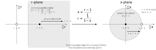
The Jaffé map sends the unwanted regular singularity $r=0$ to $x=\infty$ and compacts $1\leq r<\infty$ into $0\leq x<1$. The irregular endpoint is now the boundary point $x=1$; it has not become an ordinary point of the equation.

That last sentence is the essential caveat. Convergence for every $|x|<1$ does not imply convergence at $x=1$. Endpoint admissibility remains a large-order question about the coefficient sequence.

The Schwarzschild Jaffé–Leaver series

A historical example makes the geometry concrete without requiring the later black-hole chapter. Adopt the time dependence $\ee^{-\ii\omega t}$, set

$$\varrho=-\ii\omega, \qquad \sigma=s^2-1,$$

and let $s=0,1,2$ denote the magnitude of the field spin. In units $2M=1$, Leaver’s Schwarzschild radial equation is

$$\begin{aligned} 0 ={}& r(r-1)\psi''+\psi'\\ &-\left[ \frac{\varrho^2r^3}{r-1} +\ell(\ell+1)\right.\\ &\left.\qquad -\frac{\sigma}{r} \right]\psi. \end{aligned}$$

The endpoint-factored expansion is

$$\begin{aligned} \psi(r) ={}& (r-1)^\varrho r^{-2\varrho} \ee^{-\varrho(r-1)}\\ &\times \sum_{n=0}^{\infty} a_n \left( \frac{r-1}{r} \right)^n. \end{aligned}$$

At the horizon it has the chosen branch $(r-1)^\varrho$. At large $r$, its prefactor behaves as

$$r^{-\varrho}\ee^{-\varrho r}$$

up to an $r$-independent factor. Substitution gives

$$\mathsf A_na_{n+1} +\mathsf B_na_n +\mathsf C_na_{n-1} =0, \qquad a_{-1}=0,$$

with

$$\mathsf A_n = (n+1)(n+2\varrho+1),$$ $$\begin{aligned} \mathsf B_n = -\bigl[ &2n^2 +(8\varrho+2)n\\ &+8\varrho^2+4\varrho +\ell(\ell+1)-\sigma \bigr], \end{aligned}$$

and

$$\mathsf C_n = (n+2\varrho)^2-s^2.$$

The first equation,

$$\mathsf A_0a_1+\mathsf B_0a_0=0,$$

fixes $a_1/a_0$. It does not decide whether the resulting sequence is the one admissible at $x=1$.

A finite-point convergence test

Choose

$$\begin{aligned} \varrho&=\frac14, & \ell&=2,\\ s&=2, & \sigma&=3,\\ a_0&=1. \end{aligned}$$

This is an algebraic unit test, not a quasinormal frequency. Forward recurrence gives

$$a_1=3, \qquad a_2=\frac{133}{20}, \qquad a_3=\frac{5183}{420}.$$

For the power-series core

$$S_N(x)=\sum_{n=0}^{N}a_nx^n,$$

the partial sums are:

$N$	$S_N(1/2)$, corresponding to $r=2$	$S_N(4/5)$, corresponding to $r=5$
$20$	$10.3033116514$	$287.367689374$
$40$	$10.3051588508$	$445.287451164$
$80$	$10.3051588755$	$467.762879459$
$160$	$10.3051588755$	$467.861542284$

Every displayed point lies inside $|x|<1$, but convergence slows markedly as $x$ approaches one. At $x=1$, the same partial sums grow from approximately $7.2\times10^3$ at $N=20$ to $2.7\times10^9$ at $N=160$. The prefactor has the desired candidate exponential, yet this generic forward-generated sequence fails the remote endpoint condition.

Factoring an exponential selects a formal branch of the ansatz. It does not by itself suppress the other exact solution after the infinite sum is taken. The missing condition is recurrence minimality, developed on the next page.

Leaver-type special-function bases

Power functions are not the only basis in which a differential operator acts bandedly. Let

$$y(z) = P(z) \sum_{n\in I} a_n\phi_{n+\nu}(z),$$

where $P$ contains declared gauges and endpoint powers. Suppose, for a general basis index $k$,

$$\mathcal L\!\left(P\phi_k\right) = P\left( A_k\phi_{k-1} +B_k\phi_k +C_k\phi_{k+1} \right).$$

Exact coefficient comparison yields

$$A_{n+\nu+1}a_{n+1} +B_{n+\nu}a_n +C_{n+\nu-1}a_{n-1} =0.$$

This operator viewpoint explains several common constructions:

• $\phi_n=x^n$ gives a Jaffé power series.
• Gauss-hypergeometric or Jacobi bases retain more of a Fuchsian operator; the Heun expansions in DLMF §31.11 are examples.
• Confluent-hypergeometric and Coulomb wave bases absorb a rank-one irregular exponential and power. Leaver’s 1986 expansions for the generalized spheroidal equation are the canonical reference.

The index set is part of the representation. For a one-sided series $I=\mathbb Z_{\geq0}$, the $n=0$ term must not leave an uncancelled $\phi_{\nu-1}$ contribution. For $a_0\neq0$, this is the left-termination condition $A_\nu=0$. A two-sided series uses $I=\mathbb Z$ and usually a characteristic exponent $\nu$; it has no artificial boundary value $a_{-1}=0$.

Special functions do not guarantee convergence by their name. One must combine coefficient asymptotics with uniform estimates for $\phi_{n+\nu}(z)$ in the stated domain. A series of regular confluent hypergeometric functions, an irregular-function series, and a Coulomb-wave series can have different domains even when their coefficients satisfy proportional recurrences.

Evaluate the representation, not just the coefficients

For a power series

$$S_N(x)=\sum_{n=0}^{N}a_nx^n,$$

Horner evaluation can accumulate the value and derivative together. Start with

$$S_N=a_N, \qquad D_N=0,$$

and for $k=N-1,\ldots,0$ use

$$\begin{aligned} D_k&=S_{k+1}+xD_{k+1},\\ S_k&=a_k+xS_{k+1}. \end{aligned}$$

Then $S_0=S_N(x)$ and $D_0=S_N'(x)$. The derivative of the full solution also includes the prefactor and coordinate derivative:

$$y' = P'S_N +P\,S_N'(x)x'(z).$$

For the Jaffé variable, $x'(r)=r^{-2}$. Omitting this factor corrupts the jet even when the series value is correct.

If a proved bound

$$\left| \frac{a_{n+1}x^{n+1}}{a_nx^n} \right| \leq\tau<1$$

holds for every $n\geq N+1$, then

$$\left| S(x)-S_N(x) \right| \leq \frac{ |a_{N+1}x^{N+1}| }{ 1-\tau }.$$

One observed last-term ratio is not such a proof. A reliable computation also checks the ODE residual of the truncated representation and repeats with larger $N$. A small residual at one finite point still says nothing by itself about convergence at the boundary $x=1$.

Representation and status ledger

Claim	Correct status
Recurrence obtained by exact substitution	Exact in the declared convention
Frobenius sum strictly inside its proved disk	Convergent
Jaffé sum for $	x
Jaffé value at $x=1$	Undecided until coefficient-tail analysis is supplied
A finite $N$ partial sum	Computed approximation
Desired exponential written in the prefactor	Candidate endpoint branch, not a completed boundary condition
Special-function series with a short recurrence	Formal representation until convergence is proved

Every published expansion should record:

1. the exact equation convention and parameter tuple;
2. gauge and coordinate maps, including their inverses;
3. exponent, logarithm branch, irregular sector, and lateral choice;
4. one- or two-sided index set and normalization such as $a_0=1$;
5. recurrence coefficients and exceptional indices;
6. a proved convergence region, with its boundary kept separate; and
7. truncation, precision, residual, and independent evaluation checks.

Common pitfalls

Treating a prefactor as a boundary condition. An exponential and power select the intended formal branch. The coefficient sum can still reconstruct the unwanted exact solution unless the appropriate recurrence tail is selected.

Replacing an open disk by a closed disk. Convergence for $|x|<1$ does not include $x=1$. The compactified irregular endpoint requires a separate boundary convergence theorem.

Calling every adapted series “Leaver’s series.” Jaffé power series, Baber–Hassé modifications, Coulomb-wave series, and confluent-hypergeometric series are related but distinct representations. State the basis.

Forgetting transformed derivatives. Under $x=1-z$, $y_z=-y_x$; under $x=(r-1)/r$, $x_r=r^{-2}$. A correct value with the wrong derivative gives a wrong Wronskian.

Generating through an exceptional index. If the leading recurrence coefficient vanishes, forward division is invalid. Revisit the exponent, resonance, left termination, or parameter limit.

Equating forward recurrence with the desired tail. Forward propagation usually finds the dominant coefficient sequence. Whether the boundary requires the dominant or minimal sequence is a separate question.

Inferring convergence from a short recurrence. Tridiagonality is an algebraic property. Convergence also depends on coefficient growth and basis functions.

Using a generic confluent ansatz at a degenerate parameter. Static, extremal, or further-confluent limits can change the irregular type. Take the limit at the equation and normalization level before reusing a recurrence.

Exercises

1. Derive the general-Heun recurrence

Multiply the general Heun equation by $z(z-1)(z-a)$ and derive $\mathsf A_n$, $\mathsf B_n$, and $\mathsf D_n$. Check the two indicial roots.

Solution

The derivative coefficient is

$$\begin{aligned} B(z) ={}& \gamma(z-1)(z-a)\\ &+\delta z(z-a)\\ &+\epsilon z(z-1). \end{aligned}$$

Using the Fuchs relation,

$$B(z) = (\alpha+\beta+1)z^2 -\Xi z+\gamma a.$$

In the coefficient of $z^{n+\rho-1}$, the $az\,y''$ and $\gamma a\,y'$ terms multiply $c_n$; the $z^2$ and $z$ terms multiply $c_{n-1}$; and the $z^3$, $z^2$, and $\alpha\beta z$ terms multiply $c_{n-2}$. This gives

$$\mathsf A_n = a(n+\rho)(n+\rho+\gamma-1),$$ $$\begin{aligned} \mathsf B_n ={}& -(1+a)(n+\rho-1)(n+\rho-2)\\ &-\Xi(n+\rho-1)-q, \end{aligned}$$

and

$$\mathsf D_n = (n+\rho+\alpha-2) (n+\rho+\beta-2).$$

At $n=0$, only $\mathsf A_0c_0$ remains, so $\rho(\rho+\gamma-1)=0$.

2. Transform the right Frobenius chart

Set $x=1-z$ in the general Heun equation. Derive the transformed parameters and the sign relating $x$- and $z$-derivatives.

Solution

Since $y_z=-y_x$ and $y_{zz}=y_{xx}$, the derivative coefficient becomes

$$\frac{\delta}{x} +\frac{\gamma}{x-1} +\frac{\epsilon}{x-(1-a)}.$$

The potential term becomes

$$\frac{ \alpha\beta x-(\alpha\beta-q) }{ x(x-1)(x-(1-a)) }.$$

Thus

$$(a,q,\gamma,\delta,\epsilon) \mapsto (1-a,\alpha\beta-q,\delta,\gamma,\epsilon).$$

Every right-chart derivative inserted into a $z$-jet acquires the minus sign $\dd/\dd z=-\dd/\dd x$.

3. Audit the Heun determinant without matching

For unit-leading exponents $0,1-\gamma$ at zero and $0,1-\delta$ at one, derive the exact determinant of $C_{01}$. Specialize to the test parameters.

Solution

Near zero,

$$\Wr[f_0,f_1] \sim (1-\gamma)z^{-\gamma}.$$

Near one, with $x=1-z$,

$$\Wr[g_0,g_1] \sim -(1-\delta)x^{-\delta}.$$

Multiplication by $\mu=z^\gamma(1-z)^\delta(a-z)^\epsilon$ gives the Abel constants

$$\begin{aligned} \mathcal W_0 &= (1-\gamma)a^\epsilon,\\ \mathcal W_1 &= -(1-\delta)(a-1)^\epsilon. \end{aligned}$$

Hence

$$\det C_{01} = -\frac{1-\delta}{1-\gamma} \left( \frac{a-1}{a} \right)^\epsilon.$$

At $a=2$, $\gamma=1/2$, $\delta=2/3$, and $\epsilon=3/4$, this is $-2^{1/4}/3$.

4. Prove the Jaffé domain map

Show that $x=(r-1)/r$ maps $\operatorname{Re}r>1/2$ biholomorphically to the unit disk. Locate $r=0,1,\infty$.

Solution

For finite nonzero $r$,

$$|x|<1 \iff |r-1|^2<|r|^2.$$

Writing $r=u+\ii v$ gives

$$(u-1)^2+v^2<u^2+v^2 \iff u>\frac12.$$

The inverse is $r=1/(1-x)$, so the map is biholomorphic between the two domains. Direct substitution gives $r=1\mapsto0$, $r\to\infty\mapsto1$, and $r=0\mapsto\infty$ on the Riemann sphere.

5. Reproduce the first Schwarzschild coefficients

Use $\varrho=1/4$, $\ell=2$, $s=2$, and $a_0=1$ to compute $a_1,a_2,a_3$. Why does this calculation not define a quasinormal mode?

Solution

At $n=0$,

$$\mathsf A_0=\frac32, \qquad \mathsf B_0=-\frac92,$$

so $a_1=3$. Substitution at $n=1$ and $n=2$ gives

$$a_2=\frac{133}{20}, \qquad a_3=\frac{5183}{420}.$$

The horizon condition fixed the left end of the coefficient sequence, but no condition has yet been imposed on its $n\to\infty$ tail. Indeed, the partial sums diverge at $x=1$. A quasinormal mode requires the recurrence sequence compatible with the remote outgoing boundary condition.

6. A tridiagonal special-function basis

Assume the displayed three-term action of $\mathcal L$ on $P\phi_k$ and the series in $\phi_{n+\nu}$. Derive the coefficient recurrence and state the extra condition required for a one-sided series.

Solution

In the coefficient of $\phi_{n+\nu}$, contributions come from the lower basis-index term in $a_{n+1}\mathcal L(P\phi_{n+\nu+1})$, the middle term in $a_n\mathcal L(P\phi_{n+\nu})$, and the upper basis-index term in $a_{n-1}\mathcal L(P\phi_{n+\nu-1})$. Hence

$$A_{n+\nu+1}a_{n+1} +B_{n+\nu}a_n +C_{n+\nu-1}a_{n-1} =0.$$

For $n\geq0$, the action at the left edge must not create an uncancelled $\phi_{\nu-1}$ term. For $a_0\neq0$, this requires $A_\nu=0$, or an equivalent left-termination condition after reindexing the basis. A two-sided series has no such artificial edge.

7. When does the geometric tail bound apply?

Prove the displayed remainder bound. Explain why checking only the last two computed terms is insufficient.

Solution

If every subsequent term $t_n=a_nx^n$ obeys $|t_{n+1}|\leq\tau|t_n|$ with $\tau<1$, then

$$\begin{aligned} |S-S_N| &\leq \sum_{j=1}^{\infty}|t_{N+j}|\\ &\leq |t_{N+1}| \sum_{j=0}^{\infty}\tau^j\\ &= \frac{|t_{N+1}|}{1-\tau}. \end{aligned}$$

One observed ratio constrains only one pair of terms. A recurrence can have pre-asymptotic transients, cancellation, or a change from apparent decay to growth. A proof needs a uniform tail bound or a theorem about the recurrence solution being used.

References

• NIST Digital Library of Mathematical Functions, §2.7, Differential Equations, for Fuchs–Frobenius convergence, resonance, and irregular asymptotic status.
• NIST Digital Library of Mathematical Functions, §31.11, Expansions in Series of Hypergeometric Functions, for problem-adapted Heun bases and their convergence regions.
• NIST Digital Library of Mathematical Functions, §31.12, Confluent Forms of Heun’s Equation, for canonical confluent-Heun conventions.
• NIST Digital Library of Mathematical Functions, §31.18, Methods of Computation, for local series, numerical continuation, matching, and continued fractions.
• G. Jaffé, “Zur Theorie des Wasserstoffmolekülions,” Zeitschrift für Physik 87 (1934), 535–544, DOI: 10.1007/BF01333263.
• W. G. Baber and H. R. Hassé, “The Two Centre Problem in Wave Mechanics,” Proceedings of the Cambridge Philosophical Society 31 (1935), 564–581, DOI: 10.1017/S0305004100013566.
• E. W. Leaver, “An Analytic Representation for the Quasi-Normal Modes of Kerr Black Holes,” Proceedings of the Royal Society A 402 (1985), 285–298, DOI: 10.1098/rspa.1985.0119.
• E. W. Leaver, “Solutions to a Generalized Spheroidal Wave Equation: Teukolsky’s Equations in General Relativity, and the Two-Center Problem in Molecular Quantum Mechanics,” Journal of Mathematical Physics 27 (1986), 1238–1265, DOI: 10.1063/1.527130.
• W. Gautschi, “Computational Aspects of Three-Term Recurrence Relations,” SIAM Review 9 (1967), 24–82, DOI: 10.1137/1009002.
• L. J. El-Jaick and B. D. B. Figueiredo, “Confluent Heun Equations: Convergence of Solutions in Series of Coulomb Wavefunctions,” Journal of Physics A 46 (2013), 085203, DOI: 10.1088/1751-8113/46/8/085203.