The A₁ TQ, Quantum-Wronskian, and Y-System Relations

The previous page supplied the model, state, spectral scale, and normalization needed to call two radial determinants Baxter $Q$-functions. The next task is algebraic but phase-sensitive: turn the three-sector Stokes relation into the rank-one $TQ$ equation, use the two origin lines together to obtain the quantum Wronskian, and use four sectorial lines to generate the fusion and $Y$-systems.

All three steps are identities in a two-dimensional solution space. What changes is the projection. One origin line produces one $TQ$ equation; both origin lines produce the quantum Wronskian; four infinity lines produce the fused $T$-system. The ODE identities are exact. Their names as transfer functions, Baxter functions, Bethe equations, and $Y$-functions use the model-specific dictionary fixed on Page 4.

Throughout, take $M>1$ and a nonexceptional twist in the sense of Page 4. Put

$$q:=\mathfrak q=\omega=\ee^{\pi\ii/(M+1)}, \qquad s=v_ME, \qquad \ee^{2\pi\ii p}=\omega^{l+1/2}.$$

Here “$A_1$” refers to the rank-one Baxter problem: a second-order ODE, two complementary $Q$-branches, and one elementary transfer function. It does not mean that every fused $Y$-system below has only one node.

The functional system

Define the entire transfer eigenvalue by

$$T(s,p) := T_{\mathrm{BLZ}}(\sqrt{s},p) = C\!\left(\frac{s}{v_M},l\right).$$

Then the two normalized Baxter functions satisfy

$$\begin{aligned} T(s,p)Q_+(s,p) ={}& \ee^{-2\pi\ii p}Q_+(q^{-2}s,p) \\ &+ \ee^{2\pi\ii p}Q_+(q^2s,p), \\ T(s,p)Q_-(s,p) ={}& \ee^{2\pi\ii p}Q_-(q^{-2}s,p) \\ &+ \ee^{-2\pi\ii p}Q_-(q^2s,p). \end{aligned}$$

Their normalized quantum Wronskian is

$$\begin{aligned} &\ee^{2\pi\ii p} Q_+(qs,p)Q_-(q^{-1}s,p) \\ &\quad- \ee^{-2\pi\ii p} Q_+(q^{-1}s,p)Q_-(qs,p) \\ &=2\ii\sin(2\pi p). \end{aligned}$$

For a root with $Q_\pm(q^{-2}s_i^\pm,p)\ne0$, evaluating $TQ$ at $Q_\pm(s_i^\pm,p)=0$ gives

$$\frac{Q_\pm(q^2s_i^\pm,p)} {Q_\pm(q^{-2}s_i^\pm,p)} = -\ee^{\mp4\pi\ii p}.$$

Finally, the fused functions obey

$$T_{n/2}(q^{-1}s,p)T_{n/2}(qs,p) = 1+T_{(n-1)/2}(s,p)T_{(n+1)/2}(s,p), \qquad n\geq1,$$

and therefore

$$Y_n(q^{-1}s,p)Y_n(qs,p) = \bigl(1+Y_{n-1}(s,p)\bigr) \bigl(1+Y_{n+1}(s,p)\bigr), \qquad n\geq1.$$

The $TQ$ relation is a finite-difference identity among entire functions of the spectral variable. It is not the original differential equation in $x$: its right-hand side evaluates the same $Q$-branch at two rotated spectral arguments.

Status ledger

Statement	Status
Projected Stokes relations for the raw Wronskians	Exact ODE identities
Normalized $TQ$ equations and quantum Wronskian	Exact ODE identities at nonexceptional parameters after the Page 4 normalization
Identification $C=T$, $D_-=Q_+$, and $D_+=Q_-$	Model-specific BLZ ODE/IM correspondence
Root phase constraint	Algebraic consequence of $TQ$; called a Bethe equation after the model and state are declared
Fused $T$-system and $Y$-system	Exact Wronskian and Plücker algebra for the ODE fusion functions
Finite Dynkin-diagram truncation	Requires additional finite-cover or monodromy closure; not generic in $M$ and $l$
TBA integral equations from the $Y$-system	Require analyticity, nonzero, asymptotic, strip, and contour data; deferred to Chapter 13
Exact quantization from paired Wronskians	Deferred to Page 6

A shift ledger prevents factor-of-two errors

The BLZ operator formulas are naturally written in $\lambda$, while the ODE determinants are entire in

$$s=\lambda^2.$$

Every multiplicative shift is therefore squared when transferred to $s$:

Identity	Shift in $\lambda$	Shift in $s$
$TQ$	$q^{\pm1}\lambda$	$q^{\pm2}s$
quantum Wronskian	$q^{\pm1/2}\lambda$	$q^{\pm1}s$
fused $T$- and $Y$-systems	$q^{\pm1/2}\lambda$	$q^{\pm1}s$

This table explains why $q^2$ appears in the Bethe equation but only $q$ appears in the quantum Wronskian and $Y$-system. Changing the spectral coordinate without changing the shifts is one of the most common convention errors in ODE/IM calculations.

There is a second normalization distinction. In a standard operator gauge, the BLZ relation is phase-free:

$$\begin{aligned} \mathbf T(\lambda)\mathbf Q_\pm(\lambda) ={}& \mathbf Q_\pm(q^{-1}\lambda) \\ &+ \mathbf Q_\pm(q\lambda). \end{aligned}$$

On the highest-weight state, the raw matrix element contains a convention-dependent monomial in $\lambda$. Stripping that monomial to obtain $A_\pm$, normalizing at zero, and then setting $s=\lambda^2$ produces the phases $\ee^{\pm2\pi\ii p}$ in the scalar equations on this page. Thus a raw ODE connection Wronskian, an unstripped operator matrix element, and a normalized scalar $Q$-function are three different gauges. The displayed scalar equations fix the gauge actually used.

Projecting the three-sector relation gives TQ

Use the Page 2 adjacent normalization

$$\Wr[y_k,y_{k+1}]=2\ii$$

and the homogeneous Stokes relation

$$C(E,l)y_0=y_{-1}+y_1.$$

Let

$$a=l+\frac12.$$

The Page 3 rotation law and the Page 4 Frobenius lines give

$$\Wr[y_k,\psi_\pm](E,l) = \omega^{\pm ka} \Delta_{\mp}(\omega^{2k}E,l).$$

Take the Wronskian of the Stokes relation with $\psi_+$ and then with $\psi_-$. Bilinearity gives the two raw determinant equations

$$\begin{aligned} C(E,l)\Delta_-(E,l) ={}& \omega^{-a}\Delta_-(\omega^{-2}E,l) \\ &+ \omega^a\Delta_-(\omega^2E,l), \\ C(E,l)\Delta_+(E,l) ={}& \omega^a\Delta_+(\omega^{-2}E,l) \\ &+ \omega^{-a}\Delta_+(\omega^2E,l). \end{aligned}$$

Dividing each line by its own nonzero value at $E=0$ changes neither coefficient. The Page 4 passport then turns $\omega^{\pm a}$ into $\ee^{\pm2\pi\ii p}$ and $\omega^{\pm2}E$ into $q^{\pm2}s$. This is exactly the pair of $TQ$ relations in the result box.

Setting $s=0$ in either line supplies a quick normalization audit:

$$T(0,p) = \ee^{-2\pi\ii p}+\ee^{2\pi\ii p} = 2\cos(2\pi p).$$

The same answer from $Q_+$ and $Q_-$ is necessary because both normalized branches share one transfer eigenvalue. They do not obey literally identical scalar difference operators: stripping the two opposite highest-weight monomials produces the opposite twist phases printed above. Their monomial-dressed operator forms obey the common phase-free relation.

Zeros impose the Bethe phase equation

Let $s_i^\pm$ be a zero of $Q_\pm$. Evaluating the corresponding $TQ$ line at $s=s_i^\pm$ first gives the denominator-free identity

$$\begin{aligned} 0 ={}& \ee^{\mp2\pi\ii p}Q_\pm(q^{-2}s_i^\pm,p) \\ &+ \ee^{\pm2\pi\ii p}Q_\pm(q^2s_i^\pm,p). \end{aligned}$$

If $Q_\pm(q^{-2}s_i^\pm,p)\ne0$, division yields

$$\frac{Q_\pm(q^2s_i^\pm,p)} {Q_\pm(q^{-2}s_i^\pm,p)} = -\ee^{\mp4\pi\ii p}.$$

For $M>1$, a generic simple divisor with no shifted-root collision can be inserted into the genus-zero products from Page 4:

$$Q_\pm(s,p) = \prod_{n=0}^{\infty} \left(1-\frac{s}{s_n^\pm}\right).$$

The root equation becomes

$$\prod_{n=0}^{\infty} \frac{s_n^\pm-q^2s_i^\pm} {s_n^\pm-q^{-2}s_i^\pm} = -\ee^{\mp4\pi\ii p}.$$

The factor with $n=i$ is included. It equals $-q^2$, so deleting it silently changes the phase convention. The ratio written in the opposite order gives the reciprocal phase; neither form is meaningful until the direction of the ratio is printed.

This equation is necessary for the chosen vacuum root set. By itself it does not prove existence, admissibility, uniqueness, or completeness of solutions. Those questions require the analytic passport and, for integral-equation methods, the strip and contour data developed in Chapter 13.

The second origin line fixes the quantum Wronskian

The two Frobenius lines now enter simultaneously. In the fixed $\{\psi_-,\psi_+\}$ basis, the rotated canonical solution is

$$\begin{aligned} (2l+1)y_k ={}& \omega^{ka}\Delta_-(\omega^{2k}E,l)\psi_- \\ &- \omega^{-ka}\Delta_+(\omega^{2k}E,l)\psi_+. \end{aligned}$$

Take the Wronskian of the $k=0$ and $k=1$ formulas, use

$$\Wr[\psi_-,\psi_+]=2l+1, \qquad \Wr[y_0,y_1]=2\ii,$$

and shift $E\mapsto\omega^{-1}E$. The raw identity is

$$\begin{aligned} &\omega^a \Delta_-(\omega E,l)\Delta_+(\omega^{-1}E,l) \\ &\quad- \omega^{-a} \Delta_-(\omega^{-1}E,l)\Delta_+(\omega E,l) \\ &=2\ii(2l+1). \end{aligned}$$

Page 4 established

$$\Delta_-(0,l)\Delta_+(0,l) = \frac{2l+1}{\sin(2\pi p)}.$$

Divide by this product and use $s=v_ME$. The result is the normalized quantum Wronskian

$$\begin{aligned} &\ee^{2\pi\ii p} Q_+(qs,p)Q_-(q^{-1}s,p) \\ &\quad- \ee^{-2\pi\ii p} Q_+(q^{-1}s,p)Q_-(qs,p) \\ &=2\ii\sin(2\pi p). \end{aligned}$$

At $s=0$, this reduces to

$$\ee^{2\pi\ii p}-\ee^{-2\pi\ii p} = 2\ii\sin(2\pi p),$$

so the right-hand side audits both the phase and the zero normalization. The raw constant $2\ii(2l+1)$ and the normalized constant $2\ii\sin(2\pi p)$ must not be interchanged. At exceptional twists, including the coalescent point $p=0$, the naive normalized pair can degenerate and a limiting or derivative relation is required.

Despite its name, this quantum Wronskian is now a bilinear finite-difference invariant in the spectral variable, inherited from spatial Wronskians. It is neither an $x$-Wronskian at a fixed spectral value nor, by itself, a quantization condition. Page 6 must still declare boundary or sector data and impose a zero or compatibility condition to select a spectrum.

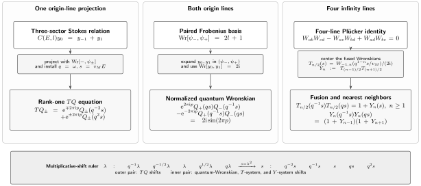
Three projections of the same two-dimensional solution geometry. The shift ruler is part of the data: a $q$-shift in $\lambda$ becomes a $q^2$-shift in $s$, whereas half-shifts in $\lambda$ become $q$-shifts in $s$. The integrable names enter only after the Page 4 passport is installed. The compact figure suppresses the fixed labels $p$ and $l$.

Plücker closure generates the fusion hierarchy

For any four solutions of a second-order equation, their Wronskians obey the Plücker identity

$$W_{ab}W_{cd} -W_{ac}W_{bd} +W_{ad}W_{bc} =0, \qquad W_{jk}:=\Wr[y_j,y_k].$$

Define the fused ODE coefficients

$$C_k^{(n)}(E,l) := \frac{1}{2\ii}W_{k-1,k+n}(E,l), \qquad n=0,1,2,\ldots.$$

Thus $C_k^{(0)}=1$ and $C_k^{(1)}=C_k$. Center the energy arguments and apply the ODE/IM name by setting

$$T_{n/2}(s,p) := C_0^{(n)}\!\left( q^{-n+1}\frac{s}{v_M},l \right).$$

In particular,

$$T_0=1, \qquad T_{1/2}=T.$$

For $n\geq1$, choose $(a,b,c,d)=(-1,0,n,n+1)$ in the Plücker identity. After using rotation covariance to center every energy and using $W_{k,k+1}=2\ii$, one obtains the uncentered relation

$$\begin{aligned} C_0^{(n)}(E)C_1^{(n)}(E) ={}& 1+C_0^{(n+1)}(E)C_1^{(n-1)}(E), \\ C_1^{(m)}(E) ={}& C_0^{(m)}(\omega^2E). \end{aligned}$$

Now put $E=q^{-n}s/v_M$ and apply the centered definition term by term. This gives

$$\begin{aligned} &T_{n/2}(q^{-1}s,p)T_{n/2}(qs,p) \\ &\qquad= 1+ T_{(n-1)/2}(s,p)T_{(n+1)/2}(s,p), \qquad n\geq1. \end{aligned}$$

This is the rank-one fusion $T$-system. It is not an independent dynamical assumption: on the ODE side it is a centered four-Wronskian identity.

The same basis expansion gives a fused bilinear that displays the two $Q$-functions explicitly. With $\theta=2\pi p$,

$$\begin{aligned} &2\ii\sin\theta\;T_{n/2}(s,p) \\ &= \ee^{\ii(n+1)\theta} Q_+(q^{n+1}s,p)Q_-(q^{-n-1}s,p) \\ &\quad- \ee^{-\ii(n+1)\theta} Q_+(q^{-n-1}s,p)Q_-(q^{n+1}s,p), \qquad n\geq0. \end{aligned}$$

The case $n=0$ is the normalized quantum Wronskian, while $n=1$ reconstructs the elementary transfer function. At $\sin\theta=0$, the direct ODE Wronskian definition must be retained and the quotient interpreted only after regularization. Page 6 uses paired members of this hierarchy as spectral conditions.

Y-functions put fusion in nearest-neighbor form

For $n\geq1$, define

$$Y_n(s,p) := T_{(n-1)/2}(s,p)T_{(n+1)/2}(s,p), \qquad Y_0:=0.$$

The $T$-system first says

$$1+Y_n(s,p) = T_{n/2}(q^{-1}s,p)T_{n/2}(qs,p).$$

Multiply the definitions of $Y_n(q^{-1}s)$ and $Y_n(qs)$, then apply the $T$-system once at each neighboring fusion index. The factors regroup into

$$\begin{aligned} Y_n(q^{-1}s,p)Y_n(qs,p) ={}& \bigl(1+Y_{n-1}(s,p)\bigr) \\ &\times \bigl(1+Y_{n+1}(s,p)\bigr). \end{aligned}$$

This is the nearest-neighbor $Y$-system. Algebra alone does not turn it into a thermodynamic Bethe ansatz. Taking logarithms, Fourier inverting the shifts, and choosing integration contours all require control of zeros, poles, branches, asymptotics, and analyticity strips.

Finite chains require monodromy closure

For generic real $M$ and generic $l$, the fusion hierarchy need not close after finitely many steps. A simple finite case, fully aligned with the even-degree return convention of Page 3, occurs at $l=0$ and integer $M>1$. The rotated canonical lines then close on the relevant finite cover, and

$$T_M(s)=1, \qquad T_{M+1/2}(s)=0,$$

so

$$Y_0=Y_{2M}=0.$$

The remaining nodes form the finite $A_{2M-1}$ $Y$-system. This subscript is the Dynkin-diagram size of the truncated fusion problem; it is distinct from the rank-one label $A_1$ attached to the elementary Baxter equation.

There is a useful zero-spectral check. Since shifts disappear at $s=0$, the $T$-system with $T_{1/2}(0)=2\cos(2\pi p)$ has the solution

$$T_{n/2}(0,p) = \frac{\sin\bigl(2\pi(n+1)p\bigr)} {\sin(2\pi p)}.$$

For $l=0$, one has $2\pi p=\pi/[2(M+1)]$, and hence $T_M(0)=1$ and $T_{M+1/2}(0)=0$. This checks the finite-cover result at one spectral point; it does not prove functional truncation without the monodromy argument.

For the quartic oscillator, $M=2$ and $p=1/12$. The complete zero-spectral fusion audit is

$$\bigl( T_0,T_{1/2},T_1,T_{3/2},T_2,T_{5/2} \bigr)(0) = \bigl(1,\sqrt3,2,\sqrt3,1,0\bigr).$$

The terminal zero is the functional-truncation endpoint, while the three interior $Y$-nodes form $A_3$.

Common pitfalls

Using the same shift in lambda and s. The $TQ$ equation shifts $\lambda$ by $q^{\pm1}$ and therefore shifts $s$ by $q^{\pm2}$. The quantum Wronskian and $Y$-system use half-shifts in $\lambda$, hence $q^{\pm1}$ in $s$.

Keeping the raw Wronskian constant after normalization. The raw ODE identity has right-hand side $2\ii(2l+1)$. Dividing by the two zero-energy connection coefficients changes it to $2\ii\sin(2\pi p)$.

Calling the root ratio a completeness theorem. Evaluating $TQ$ at a zero gives a necessary phase equation. Completeness and admissibility need additional analytic and state data.

Assuming every Y-system truncates. Plücker gives the infinite fusion relations without a finite-cover hypothesis. A finite Dynkin diagram requires extra monodromy closure.

Exercises

1. Recover both twist phases. Starting from the rotated projection formula, derive the two raw determinant relations and identify which line maps to $Q_+$.

Solution

For $\psi_+$,

$$\Wr[y_k,\psi_+] = \omega^{ka}\Delta_-(\omega^{2k}E).$$

Projecting $Cy_0=y_{-1}+y_1$ therefore gives

$$C\Delta_- = \omega^{-a}\Delta_-(\omega^{-2}E) +\omega^a\Delta_-(\omega^2E).$$

The signs reverse for $\psi_-$. Since Page 4 identifies $Q_+=D_-$, the first line is the $Q_+$ equation. Finally $\omega^{\pm a}=\ee^{\pm2\pi\ii p}$.

2. Audit the squared coordinate. If an operator formula contains $Q(q^{-1}\lambda)$ and $Q(q\lambda)$, show what arguments appear after writing the normalized scalar function in $s=\lambda^2$.

Solution

Squaring the shifted coordinates gives

$$(q^{-1}\lambda)^2=q^{-2}s, \qquad (q\lambda)^2=q^2s.$$

Thus the entire scalar arguments are $q^{-2}s$ and $q^2s$. The same calculation sends $q^{\pm1/2}\lambda$ to $q^{\pm1}s$.

3. Derive the Bethe product. Evaluate $TQ$ at a $Q_+$ zero and insert the canonical product. Compute the factor with $n=i$.

Solution

At $Q_+(s_i^+)=0$,

$$\ee^{-2\pi\ii p}Q_+(q^{-2}s_i^+) +\ee^{2\pi\ii p}Q_+(q^2s_i^+)=0,$$

so

$$\frac{Q_+(q^2s_i^+)}{Q_+(q^{-2}s_i^+)} =-\ee^{-4\pi\ii p}.$$

The canonical product gives

$$\prod_n \frac{s_n^+-q^2s_i^+}{s_n^+-q^{-2}s_i^+} =-\ee^{-4\pi\ii p}.$$

For $n=i$, the factor is

$$\frac{1-q^2}{1-q^{-2}}=-q^2.$$

4. Normalize the quantum Wronskian. Divide the raw paired identity by the zero-energy constants and recover its exact right-hand side.

Solution

The raw right-hand side is $2\ii(2l+1)$. Page 4 gives

$$\Delta_-(0,l)\Delta_+(0,l) = \frac{2l+1}{\sin(2\pi p)}.$$

Therefore normalization changes the constant to

$$\frac{2\ii(2l+1)} {(2l+1)/\sin(2\pi p)} = 2\ii\sin(2\pi p).$$

5. Identify what the functional identities do not select. Why does the quantum Wronskian alone give neither an exact spectrum nor a TBA integral equation? List the extra data needed in each case.

Solution

The bilinear identity holds throughout the spectral family and does not choose a spectral value. Exact quantization additionally needs a declared endpoint domain or pair of recessive sectors and a zero or compatibility condition for the corresponding determinant or Wronskian. A TBA derivation instead needs an analyticity strip, zero-and-pole information, nonzero assumptions or explicit source terms, asymptotics, logarithm branches, and integration contours. Those data enter on Page 6 and in Chapter 13, respectively.

6. Derive the T-system from Plücker. Apply the four-line identity to $(-1,0,n,n+1)$ and explain the origin of the constant $1$.

Solution

Plücker gives

$$W_{-1,0}W_{n,n+1} -W_{-1,n}W_{0,n+1} +W_{-1,n+1}W_{0,n}=0.$$

Put $E_s=s/v_M$ and $F=q^{-n}E_s$. Rotation covariance identifies

$$\begin{aligned} \frac{W_{-1,n}(F)}{2\ii} &=T_{n/2}(q^{-1}s), & \frac{W_{0,n+1}(F)}{2\ii} &=T_{n/2}(qs), \\ \frac{W_{0,n}(F)}{2\ii} &=T_{(n-1)/2}(s), & \frac{W_{-1,n+1}(F)}{2\ii} &=T_{(n+1)/2}(s). \end{aligned}$$

The first Plücker product is $(2\ii)^2$. Move the middle term to the other side and divide by $(2\ii)^2$. The adjacent product becomes $1$, while the remaining product gives the neighboring fused functions. Hence

$$T_{n/2}(q^{-1}s)T_{n/2}(qs) =1+T_{(n-1)/2}(s)T_{(n+1)/2}(s).$$

7. Derive the Y-system. Starting from $Y_n=T_{(n-1)/2}T_{(n+1)/2}$, prove the nearest-neighbor relation.

Solution

Multiply the shifted definitions:

$$\begin{aligned} Y_n(q^{-1}s)Y_n(qs) ={}& \bigl[T_{(n-1)/2}(q^{-1}s) T_{(n-1)/2}(qs)\bigr] \\ &\times \bigl[T_{(n+1)/2}(q^{-1}s) T_{(n+1)/2}(qs)\bigr]. \end{aligned}$$

The $T$-system turns the first bracket into $1+Y_{n-1}(s)$ and the second into $1+Y_{n+1}(s)$.

8. Audit the quartic system. For $M=2$ and $l=0$, compute $q,p,T(0,p)$, the quantum-Wronskian constant, the two Bethe phases, and the finite $Y$-system size.

Solution

Here

$$q=\ee^{\pi\ii/3}, \qquad p=\frac1{12}.$$

Thus

$$T(0,p)=2\cos\!\left(\frac{\pi}{6}\right)=\sqrt3,$$

and the normalized quantum-Wronskian constant is

$$2\ii\sin\!\left(\frac{\pi}{6}\right)=\ii.$$

The $Q_+$ and $Q_-$ root ratios are respectively $-\ee^{-\pi\ii/3}$ and $-\ee^{\pi\ii/3}$. Since $2M=4$, the finite closure has $Y_0=Y_4=0$ and three interior nodes: the $A_3$ system.

References

• R. J. Baxter, Exactly Solved Models in Statistical Mechanics, Academic Press, 1982, Chapters 9–10, for the original transfer-matrix, $Q$-operator, and Bethe-root framework.
• V. V. Bazhanov, S. L. Lukyanov, and A. B. Zamolodchikov, “Integrable Structure of Conformal Field Theory II: Q-Operator and DDV Equation”, Communications in Mathematical Physics 190 (1997), 247–278, for the conformal $TQ$ system and quantum Wronskian.
• V. Bazhanov, S. Lukyanov, and A. Zamolodchikov, “Spectral Determinants for Schrödinger Equation and Q-Operators of Conformal Field Theory”, Journal of Statistical Physics 102 (2001), 567–576, for the normalized analytic characterization of the two vacuum Baxter functions.
• P. Dorey and R. Tateo, “On the Relation between Stokes Multipliers and the T–Q Systems of Conformal Field Theory”, Nuclear Physics B 563 (1999), 573–602, with erratum, for the projected ODE $TQ$ equations, fused Stokes functions, quantum Wronskians, and $Y$-system used here.
• P. Dorey, C. Dunning, and R. Tateo, “The ODE/IM Correspondence”, Journal of Physics A 40 (2007), R205–R283, especially Sections 5.2–5.5 for a later unified account of the functional relations and their analytic hypotheses. The phases and raw normalizations on this page follow the primary sources above.
• J. Suzuki, “Anharmonic Oscillators, Spectral Determinant and Short Exact Sequence of affine Uq(sl₂)”, Journal of Physics A 32 (1999), L183–L188, for a proof of the anharmonic-oscillator $T$-system relation from Stokes data.
• Al. B. Zamolodchikov, “On the Thermodynamic Bethe Ansatz Equations for Reflectionless ADE Scattering Theories”, Physics Letters B 253 (1991), 391–394, for the finite ADE $Y$-systems and their thermodynamic Bethe-ansatz setting.
• Y. Sibuya, Global Theory of a Second Order Linear Ordinary Differential Equation with a Polynomial Coefficient, North-Holland, 1975, for the canonical sectorial solutions and Stokes multipliers on the ODE side.