c = 1 Block Expansions of Isomonodromic Tau Functions

Near $t=0$, the generic Painlevé VI tau function is not one conformal block and not a Taylor series. It is a fractional Fourier series of complete chiral $c=1$ Virasoro blocks. Moving horizontally changes the logarithmic lift of the composite monodromy; moving vertically adds Virasoro descendants.

This page fixes every factor in that statement. The result is an exact local identity on a generic marked monodromy chart, up to the unavoidable nonzero $t$-independent JMU factor. It also gives two coefficient constructions, an explicit trace-to-twist map, a worked fractional-power example, and a two-cutoff numerical workflow.

Two indices, two truncation errors

The charge $n\in\mathbb Z$ and the descendant level $k\in\mathbb Z_{\ge0}$ are independent. A term has exponent $\kappa_n+k$, so increasing the block level at fixed $n$ cannot repair a charge truncation, and enlarging the charge window cannot repair a descendant truncation.

Status of the formula

Gamayun–Iorgov–Lisovyy stated the expansion as a claim in 2012. Iorgov–Lisovyy–Teschner derived the generic $c=1$ Fourier construction from degenerate-field monodromy, and Gavrylenko–Lisovyy proved the charged partition series from a Fredholm determinant. The formula below is therefore an established generic local identity, not merely a matched asymptotic ansatz. Exceptional Kac and resonant loci still require limits of the assembled expression.

A marked monodromy chart fixes the theorem

Use the traceless four-pole system and the exponent convention of Chapter 5:

$$\operatorname{spec}A_\nu = \left\{ +\frac{\theta_\nu}{2}, -\frac{\theta_\nu}{2} \right\}, \qquad \operatorname{tr}M_\nu = 2\cos(\pi\theta_\nu).$$

Choose a lift $\sigma_{0t}$ of the separating trace

$$\operatorname{tr}(M_0M_t) = 2\cos(\pi\sigma_{0t})$$

and define the charge lattice

$$\begin{aligned} q_n &= \sigma_{0t}+2n, \\ \Delta_\nu^{\mathrm{ext}} &= \frac{\theta_\nu^2}{4}, \\ \Delta_n^{\mathrm{int}} &= \frac{q_n^2}{4}, \qquad n\in\mathbb Z. \end{aligned}$$

The channel exponent is

$$\kappa_n := \Delta_n^{\mathrm{int}} -\Delta_0^{\mathrm{ext}} -\Delta_t^{\mathrm{ext}} = \frac{ q_n^2-\theta_0^2-\theta_t^2 }{4}.$$

The source convention uses residue eigenvalues $\pm\vartheta_\nu$ and composite lift $\rho$, so

$$\vartheta_\nu = \frac{\theta_\nu}{2}, \qquad \rho = \frac{\sigma_{0t}}{2}, \qquad \rho+n = \frac{q_n}{2}.$$

This conversion accounts for every factor of two in the formulas below.

The exact local Fourier expansion

Let

$$\widehat{\mathcal F}_1 \left( \boldsymbol\theta,q;t \right) = 1+\sum_{k\ge1} f_k(\boldsymbol\theta,q)t^k$$

be the unit-leading $0t$-channel Virasoro block with $c_{\mathrm{Vir}}=1$, external weights $\theta_\nu^2/4$, and internal weight $q^2/4$. In the Barnes normalization fixed below,

$$\begin{aligned} \tau_{\mathrm J}(t;\mathcal M) ={}& C(\mathcal M) \sum_{n\in\mathbb Z} s_{\mathrm F}^{\,n} \mathcal C_{c=1} \left( \boldsymbol\theta,q_n \right) \\ &\times t^{\kappa_n} \widehat{\mathcal F}_1 \left( \boldsymbol\theta,q_n;t \right). \end{aligned}$$

Here $C(\mathcal M)\in\mathbb C^\times$ is independent of $t$, and $s_{\mathrm F}\in\mathbb C^\times$ is the second, twist-like monodromy coordinate in this chiral normalization. This page chooses the standard unit-leading block, so the elementary factor $\mathcal E$ left schematic on page 1 is exactly $1$.

Choose $\Log t$ and $\Log(1-t)$ on a simply connected small-$t$ chart. A sufficient generic chart is

$$|\Re\sigma_{0t}|<1, \qquad \sigma_{0t}\notin\mathbb Z, \qquad s_{\mathrm F}\neq0,$$

together with nonresonant local residues and

$$\begin{aligned} \theta_0\pm\theta_t\pm\sigma_{0t} &\notin2\mathbb Z, \\ \theta_1\pm\theta_\infty\pm\sigma_{0t} &\notin2\mathbb Z, \end{aligned}$$

for all independent signs. These conditions are sufficient rather than necessary. Gavrylenko–Lisovyy state their Fredholm theorem for $0<t<1$ and a slightly larger closed lift strip; complex charts follow by analytic continuation with the marking and branches transported. Near $t=1$, use the crossed channel instead of assuming that the $t=0$ expansion remains uniformly convergent at its boundary.

Five factors with five different jobs

Factor	Meaning	Depends on $t$?	What can change it?
$C(\mathcal M)$	JMU integration constant	No	Framing and global tau normalization
$s_{\mathrm F}^{\,n}$	Twist weight of charge $n$	No	Marked monodromy and chiral normalization
$\mathcal C_{c=1}(\boldsymbol\theta,q_n)$	Barnes chiral structure factor	No	Vertex and exponent conventions
$t^{\kappa_n}$	OPE channel power	Yes	Exponent lift and $\Log t$
$\widehat{\mathcal F}_1$	Complete descendant series	Yes	Block normalization and channel

The notation $s_{\mathrm F}=\ee^{\ii\eta_{\mathrm F}}$ is convenient locally, but $\eta_{\mathrm F}$ is generally complex. It does not imply $|s_{\mathrm F}|=1$.

Barnes-G factors propagate along the charge lattice

Let $G$ denote the Barnes function,

$$G(z+1) = \Gamma(z)G(z).$$

Define a width-safe trinion product

$$\mathscr G(x,y;u) := \prod_{\epsilon,\epsilon'=\pm1} G\left( 1+ \frac{ x+\epsilon y+\epsilon'u }{2} \right).$$

The structure factor in the displayed tau formula is

$$\mathcal C_{c=1} \left( \boldsymbol\theta,u \right) = \frac{ \mathscr G(\theta_t,\theta_0;u) \mathscr G(\theta_1,\theta_\infty;u) }{ G(1+u)G(1-u) }.$$

It is an even meromorphic function:

$$\mathcal C_{c=1} \left( \boldsymbol\theta,-u \right) = \mathcal C_{c=1} \left( \boldsymbol\theta,u \right).$$

These are analytic chiral normalization factors. They are not DOZZ coefficients, and the Fourier multiplier prevents their interpretation as a product of ordinary physical Liouville three-point functions.

A Gamma-only shift audit

Repeatedly evaluating eight Barnes functions is unnecessary. Set

$$R(u) := \frac{ \mathcal C_{c=1}(\boldsymbol\theta,u+2) }{ \mathcal C_{c=1}(\boldsymbol\theta,u) }.$$

The Barnes recurrence gives

$$R(u) = R_0(u) R_{\theta_t,\theta_0}(u) R_{\theta_1,\theta_\infty}(u),$$

where

$$R_0(u) = \frac{ \Gamma(-u)\Gamma(-1-u) }{ \Gamma(1+u)\Gamma(2+u) }$$

and

$$R_{x,y}(u) = \prod_{\epsilon=\pm1} \frac{ \Gamma\left( 1+\frac{x+\epsilon y+u}{2} \right) }{ \Gamma\left( \frac{x+\epsilon y-u}{2} \right) }.$$

This recurrence is both an implementation method and a transcription check. Seed it with a direct high-precision Barnes evaluation, propagate logarithms with their complex phases, and compare an occasional direct value. If an intermediate Gamma argument crosses a pole, restart on the other side rather than multiplying formal infinities and zeros.

From trace coordinates to the Fourier multiplier

Define the remaining composite lifts by

$$\begin{aligned} \operatorname{tr}(M_0M_1) &= 2\cos(\pi\sigma_{01}), \\ \operatorname{tr}(M_1M_t) &= 2\cos(\pi\sigma_{1t}), \end{aligned}$$

and abbreviate

$$c(x) := \cos(\pi x), \qquad \chi := \sin(\pi\sigma_{0t}).$$

In the Gamayun–Iorgov–Lisovyy Barnes normalization, set

$$\begin{aligned} D_\pm ={}& \left[ c(\theta_t\mp\sigma_{0t}) -c(\theta_0) \right] \\ &\times \left[ c(\theta_1\mp\sigma_{0t}) -c(\theta_\infty) \right] \end{aligned}$$

and

$$\begin{aligned} N_\pm ={}& c(\theta_t)c(\theta_1) +c(\theta_0)c(\theta_\infty) \\ &\quad \pm\ii\chi\,c(\sigma_{01}) \\ &- \Bigl[ c(\theta_0)c(\theta_1) +c(\theta_t)c(\theta_\infty) \\ &\qquad \mp\ii\chi\,c(\sigma_{1t}) \Bigr] \ee^{\pm\pi\ii\sigma_{0t}}. \end{aligned}$$

On the chart $D_+D_-\neq0$,

$$s_{\mathrm F}^{\,\pm1} = \frac{N_\pm}{D_\pm}.$$

The Jimbo–Fricke relation makes the two signs consistent. If either $D_\pm$ vanishes, this coordinate chart has failed; the tau function need not be singular. Use another character-variety coordinate or take a controlled limit.

The Fourier variables used by Iorgov–Lisovyy–Teschner and Gavrylenko–Lisovyy differ from $s_{\mathrm F}$ by explicit chiral and trinion normalization factors. They must not be identified by name alone.

Virasoro sewing becomes a bipartition sum

The unit-leading block can be computed from Gram matrices, as in Chapter 6, or from an explicit pair of Young diagrams. For the latter, write

$$\vartheta_\nu = \frac{\theta_\nu}{2}, \qquad \rho = \frac{u}{2}.$$

For a partition $\lambda$, let

$$h_\lambda(i,j) = \lambda'_j-i+\lambda_i-j+1$$

be the hook length. Missing rows are understood to have length zero. Define

$$\begin{aligned} \mathscr W^+_{\lambda,\mu} (i,j;\rho) :={}& \frac{ \left[ (\vartheta_t+\rho+i-j)^2-\vartheta_0^2 \right] }{ h_\lambda(i,j)^2 } \\ &\times \frac{ \left[ (\vartheta_1+\rho+i-j)^2-\vartheta_\infty^2 \right] }{ \left[ \lambda'_j-i+\mu_i-j+1+2\rho \right]^2 } \end{aligned}$$

and

$$\begin{aligned} \mathscr W^-_{\mu,\lambda} (i,j;\rho) :={}& \frac{ \left[ (\vartheta_t-\rho+i-j)^2-\vartheta_0^2 \right] }{ h_\mu(i,j)^2 } \\ &\times \frac{ \left[ (\vartheta_1-\rho+i-j)^2-\vartheta_\infty^2 \right] }{ \left[ \mu'_j-i+\lambda_i-j+1-2\rho \right]^2 }. \end{aligned}$$

The bipartition weight is

$$\mathcal B_{\lambda,\mu} \left( \boldsymbol\vartheta,\rho \right) = \prod_{(i,j)\in\lambda} \mathscr W^+_{\lambda,\mu}(i,j;\rho) \prod_{(i,j)\in\mu} \mathscr W^-_{\mu,\lambda}(i,j;\rho).$$

Then

$$\begin{aligned} \widehat{\mathcal F}_1 \left( \boldsymbol\theta,u;t \right) ={}& (1-t)^{\theta_t\theta_1/2} \\ &\times \sum_{\lambda,\mu} \mathcal B_{\lambda,\mu} \left( \boldsymbol\vartheta,\rho \right) t^{|\lambda|+|\mu|}. \end{aligned}$$

The empty pair gives $1$. If the bare bipartition sum is denoted by $\mathcal Z_{\mathrm{part}}$, the exact convention bridge is

$$\widehat{\mathcal F}_1 = (1-t)^a\mathcal Z_{\mathrm{part}}, \qquad a = \frac{\theta_t\theta_1}{2}.$$

One may therefore use the alternative page-1 split $\mathcal E=(1-t)^a$ and $\widehat{\mathcal V}=\mathcal Z_{\mathrm{part}}$. This merely moves a factor inside an unchanged product; it does not alter $\tau_{\mathrm J}$ or $\partial_t\log\tau_{\mathrm J}$.

The level-one coefficient checks both constructions

The sole level-one state is $L_{-1}|\Delta_u^{\mathrm{int}}\rangle$, with

$$\Delta_u^{\mathrm{int}} = \frac{u^2}{4}, \qquad \langle\Delta_u^{\mathrm{int}}| L_1L_{-1} |\Delta_u^{\mathrm{int}}\rangle = 2\Delta_u^{\mathrm{int}}.$$

The two Ward couplings give $\Delta_u^{\mathrm{int}}+\Delta_t^{\mathrm{ext}} -\Delta_0^{\mathrm{ext}}$ and $\Delta_u^{\mathrm{int}}+\Delta_1^{\mathrm{ext}} -\Delta_\infty^{\mathrm{ext}}$. Hence

$$\widehat{\mathcal F}_1 \left( \boldsymbol\theta,u;t \right) = 1+f_1(\boldsymbol\theta,u)t+O(t^2),$$

with

$$f_1(\boldsymbol\theta,u) = \frac{ \left( u^2+\theta_t^2-\theta_0^2 \right) \left( u^2+\theta_1^2-\theta_\infty^2 \right) }{ 8u^2 }.$$

At bipartition level one, only $([1],\varnothing)$ and $(\varnothing,[1])$ contribute. Their sum is

$$\left[t\right]\mathcal Z_{\mathrm{part}} = f_1(\boldsymbol\theta,u) +\frac{\theta_t\theta_1}{2},$$

which exactly compensates the linear term of $(1-t)^a$. This is a sensitive check of insertion order, the AGT prefactor, and the factor-of-two dictionary.

The denominator $u^2$ also advertises the genericity boundary: $u=0$ must be handled as a degenerate limit, not substituted into this Gram-inverse formula.

The first frontier in the lower half-strip

Every charge–descendant cell contributes

$$s_{\mathrm F}^{\,n} \mathcal C_{c=1} \left( \boldsymbol\theta,q_n \right) f_k \left( \boldsymbol\theta,q_n \right) t^{\kappa_n+k}.$$

The difference from the central vacuum exponent is

$$\kappa_n-\kappa_0 = n^2+n\sigma_{0t}.$$

For $0<\Re\sigma_{0t}<1/2$, the first cells are therefore

Charge and level	Relative exponent	Origin
$(n,k)=(0,0)$	$0$	Central primary
$(-1,0)$	$1-\sigma_{0t}$	Neighboring exponent lift
$(0,1)$	$1$	First Virasoro descendant
$(+1,0)$	$1+\sigma_{0t}$	Other neighboring lift
$(-1,1)$	$2-\sigma_{0t}$	Descendant in the left charge sector

Define

$$\begin{aligned} r_- &:= s_{\mathrm F}^{-1} \frac{ \mathcal C_{c=1} (\boldsymbol\theta,\sigma_{0t}-2) }{ \mathcal C_{c=1} (\boldsymbol\theta,\sigma_{0t}) }, \\ r_+ &:= s_{\mathrm F} \frac{ \mathcal C_{c=1} (\boldsymbol\theta,\sigma_{0t}+2) }{ \mathcal C_{c=1} (\boldsymbol\theta,\sigma_{0t}) }. \end{aligned}$$

Factoring the central vacuum gives the audit

$$\begin{aligned} \tau_{\mathrm J} ={}& C(\mathcal M) \mathcal C_{c=1} (\boldsymbol\theta,\sigma_{0t}) t^{\kappa_0} \\ &\times \left[ 1 +r_-t^{1-\sigma_{0t}} +f_1(\boldsymbol\theta,\sigma_{0t})t {}\right. \\ &\left.\qquad +r_+t^{1+\sigma_{0t}} +\cdots \right]. \end{aligned}$$

The ellipsis is a generalized power series, not a promise that the displayed terms remain ordered outside this half-strip. On $\Re\sigma_{0t}=1/2$, the real parts of the exponents of $(+1,0)$ and $(-1,1)$ tie; the cells collide exactly at $\sigma_{0t}=1/2$. For $1/2<\Re\sigma_{0t}<1$, the latter precedes the former. Higher descendants and $|n|\ge2$ cells can also reorder when exponent real parts or coefficient magnitudes change.

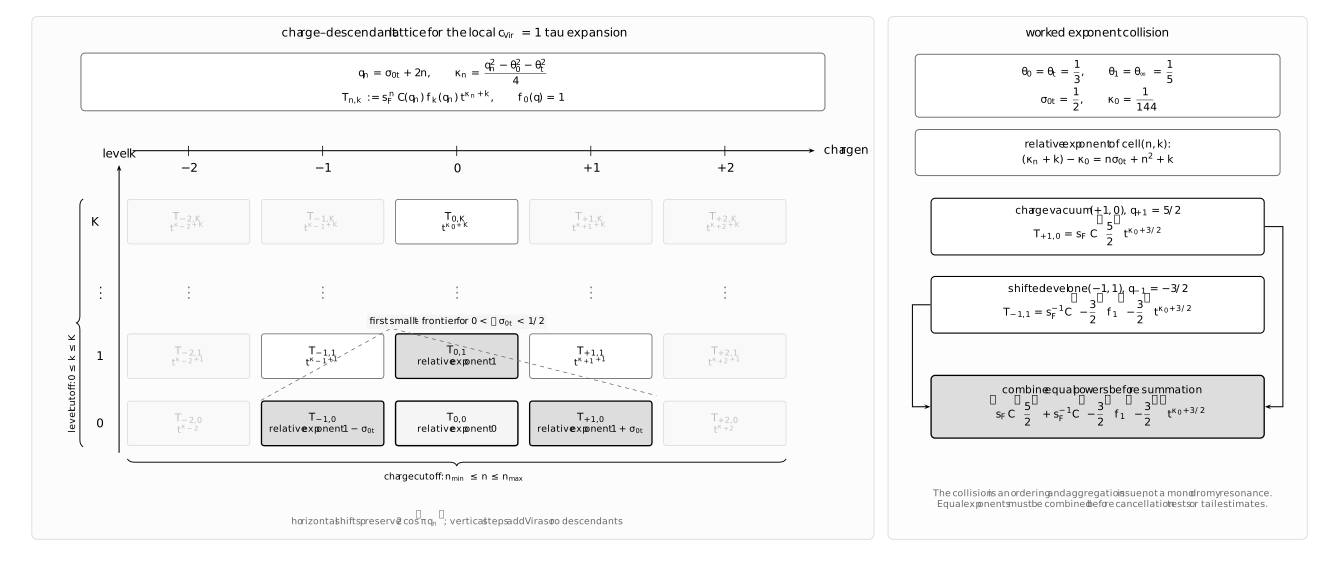
Each lattice cell carries one power $t^{\kappa_n+k}$. Horizontal motion changes the composite exponent lift while preserving its trace; vertical motion adds descendants. The highlighted lower-half-strip frontier explains why the first fractional powers come from different conformal blocks. At its boundary $\sigma_{0t}=1/2$, the cells $(+1,0)$ and $(-1,1)$ meet at relative exponent $3/2$ and must be combined.

A rational example exposes a colliding power

Choose

$$\theta_0 = \theta_t = \frac13, \qquad \theta_1 = \theta_\infty = \frac15, \qquad \sigma_{0t} = \frac12.$$

These exponent values satisfy the stated exclusions. Choose in addition generic compatible trace data, hence a finite nonzero $s_{\mathrm F}$. The paired external weights make the level-one coefficient particularly transparent:

$$f_1(\boldsymbol\theta,u) = \frac{u^2}{8}.$$

For the central sector,

$$\kappa_0 = \frac1{144}, \qquad f_1 \left( \boldsymbol\theta,\frac12 \right) = \frac1{32}.$$

The bare bipartition coefficient differs by

$$a = \frac1{30}, \qquad \left[t\right]\mathcal Z_{\mathrm{part}} = \frac1{32}+\frac1{30} = \frac{31}{480}.$$

The neighboring vacuum exponents are

$$\kappa_{-1} = \frac{73}{144} = \kappa_0+\frac12, \qquad \kappa_{+1} = \frac{217}{144} = \kappa_0+\frac32.$$

In this example,

$$\begin{aligned} r_- &= s_{\mathrm F}^{-1} \frac{ \mathcal C_{c=1}(\boldsymbol\theta,-3/2) }{ \mathcal C_{c=1}(\boldsymbol\theta,1/2) }, \\ r_+ &= s_{\mathrm F} \frac{ \mathcal C_{c=1}(\boldsymbol\theta,5/2) }{ \mathcal C_{c=1}(\boldsymbol\theta,1/2) }. \end{aligned}$$

The normalized series begins

$$\begin{aligned} \frac{ \tau_{\mathrm J} }{ C(\mathcal M) \mathcal C_{c=1}(\boldsymbol\theta,1/2) t^{1/144} } ={}& 1+r_-t^{1/2} +\frac1{32}t \\ &+ \left( r_+ +\frac9{32}r_- \right)t^{3/2} +\cdots. \end{aligned}$$

The coefficient of $t^{3/2}$ is not attached to one block. It combines the $(+1,0)$ vacuum with the $(-1,1)$ descendant, for which $f_1(\boldsymbol\theta,-3/2)=9/32$. Equal powers must be aggregated before cancellation estimates, logarithms, or error bars are formed.

The Hamiltonian differentiates the assembled sum

For the traceless JMU representative,

$$H_t := \partial_t\log\tau_{\mathrm J} = \frac{\operatorname{tr}(A_0A_t)}{t} +\frac{\operatorname{tr}(A_tA_1)}{t-1}.$$

Define the full weight of charge $n$ by

$$w_n(t) := s_{\mathrm F}^{\,n} \mathcal C_{c=1} (\boldsymbol\theta,q_n) t^{\kappa_n} \widehat{\mathcal F}_1 (\boldsymbol\theta,q_n;t).$$

Away from a zero of $\tau_{\mathrm J}$, termwise differentiation on the convergent local chart yields

$$H_t = \frac{ \displaystyle \sum_{n\in\mathbb Z} w_n \left[ \frac{\kappa_n}{t} +\partial_t \log\widehat{\mathcal F}_1 (\boldsymbol\theta,q_n;t) \right] }{ \displaystyle \sum_{n\in\mathbb Z}w_n }.$$

This is a ratio of two summed series. It is not a sum of the logarithmic derivatives of individual blocks. The factor $C(\mathcal M)$ cancels, while a zero of the tau function becomes a pole of $H_t$.

The selected-term version is width-safe:

$$\begin{aligned} tH_t = \kappa_0 +\frac{ \mathcal N_{\mathrm{front}}(t) }{ \mathcal D_{\mathrm{front}}(t) }, \end{aligned}$$

where

$$\begin{aligned} \mathcal N_{\mathrm{front}} ={}& (1-\sigma_{0t})r_-t^{1-\sigma_{0t}} \\ &+ f_1(\boldsymbol\theta,\sigma_{0t})t \\ &+ (1+\sigma_{0t})r_+t^{1+\sigma_{0t}} +\cdots, \\ \mathcal D_{\mathrm{front}} ={}& 1+r_-t^{1-\sigma_{0t}} \\ &+ f_1(\boldsymbol\theta,\sigma_{0t})t \\ &+ r_+t^{1+\sigma_{0t}} +\cdots. \end{aligned}$$

On a fixed ray, with $|\Re\sigma_{0t}|<1$ and a nonzero central coefficient,

$$\lim_{t\to0} t\,\partial_t\log\tau_{\mathrm J} = \kappa_0.$$

Two cutoffs make the series computational

A robust evaluator should retain the charge and descendant structure rather than flattening it prematurely.

1. Fix $\boldsymbol\theta$, the lift $\sigma_{0t}$, $s_{\mathrm F}$, $\Log t$, working precision, a charge window $n_{\min}\le n\le n_{\max}$, and a level cutoff $K$.
2. Evaluate one Barnes seed directly and use the Gamma shift recurrence in both directions, periodically checking against direct high-precision values.
3. Compute $f_k(\boldsymbol\theta,q_n)$ from Virasoro Gram matrices, or compute the bipartition coefficients through total size $K$.
4. Attach the exponent $\kappa_n+k$ and the complete complex amplitude to every cell.
5. Aggregate cells with equal exponents, then sum terms in increasing estimated magnitude with compensated or higher-precision arithmetic.
6. Increase $K$ and the charge window separately. A useful charge window need not be symmetric because it depends on $\Re\kappa_n$, $|s_{\mathrm F}|^n$, and the Barnes factors.
7. Supply a majorant, interval enclosure, or independently justified tail bound whenever a certified result is claimed.

The following checks isolate different errors:

Check	What it detects
Level-one Ward coefficient	Block normalization or external-label permutation
Barnes shift recurrence	Structure-factor transcription or phase error
$\sigma_{0t}\mapsto\sigma_{0t}+2$ reindexing	Charge and twist convention error
Separate level and charge-window convergence	Hidden truncation imbalance
Chapter 5 Fredholm value	Independent representation error
JMU Hamiltonian residual	Tau convention or differentiation error
Higher precision at fixed cutoffs	Roundoff and cancellation

The Fredholm comparison is genuinely independent: it reconstructs the same charged partition series from hypergeometric parametrices and principal minors, without assuming conformal field theory. For that comparison, obtain both Fourier variables from the same trace data or apply the explicit normalization conversion; do not equate the Fredholm and chiral twist symbols merely because both exponentiate a coordinate called $\eta$.

Lift changes, braids, and Kac limits are different operations

Let $\mathcal T(\sigma,s;t)$ denote the Fourier sum without the overall factor $C(\mathcal M)$. Reindexing the charge gives

$$\mathcal T \left( \sigma+2m,s;t \right) = s^{-m} \mathcal T \left( \sigma,s;t \right), \qquad m\in\mathbb Z.$$

Thus changing the logarithmic lift changes only a $t$-independent representative factor. If a fixed normalized tau is to be preserved, $C(\mathcal M)$ transforms oppositely. Evenness of the structure factor and dependence of the block on $q^2$ also give

$$\mathcal T(-\sigma,s^{-1};t) = \mathcal T(\sigma,s;t).$$

A counterclockwise circuit of $t$ around zero instead changes the branch:

$$\Log t \longmapsto \Log t+2\pi\ii.$$

Since

$$\kappa_n-\kappa_0 = n\sigma_{0t}+n^2,$$

the continued local series obeys

$$\mathcal T \longmapsto \ee^{2\pi\ii\kappa_0} \mathcal T \left( \sigma_{0t}, \ee^{2\pi\ii\sigma_{0t}}s_{\mathrm F}; t \right).$$

The common phase is branch and normalization data; the relative multiplier is the Hurwitz action on marked monodromy. This is why the expansion is not globally single-valued term by term.

Kac-degenerate cells must be assembled before taking a limit

At $c=1$, the internal Kac lattice is

$$\Delta_{\mathrm{int}} = \frac{m^2}{4}, \qquad m\in\mathbb Z.$$

Because every $q_n=\sigma_{0t}+2n$, the entire charge family meets this lattice precisely when $\sigma_{0t}\in\mathbb Z$. Then Gram inverses can have Zamolodchikov poles, Barnes factors can vanish or diverge, and charge–descendant cells collide. Moreover, $\sin(\pi\sigma_{0t})=0$, so the displayed trace-to-twist chart also degenerates.

If $\sigma_{0t}=m$, one unavoidable primary-weight partner is

$$n' = -m-n, \qquad q_{n'} = -q_n.$$

That sign partner is not the whole cancellation pattern. At $\sigma_{0t}=0$, for example, the singular level-one cell of the self-paired $q=0$ block has the same exponent as the $q=\pm2$ vacua. At $\sigma_{0t}=1$, level-two cells with $q=\pm1$ meet vacua with $q=\pm3$. The correct general procedure is therefore

$$\sigma_{0t} = m+\varepsilon \quad\longrightarrow\quad \begin{gathered} \text{assemble the full generic Fourier sum,}\\ \text{or all cells colliding at the retained powers} \end{gathered} \quad\longrightarrow\quad \varepsilon\to0.$$

Coefficients proportional to $1/\varepsilon$ can combine with $t^{\alpha\pm c\varepsilon}$ to leave $t^\alpha\Log t$. A finite limiting tau function is possible but is not automatic. Local Frobenius resonance $\theta_\nu\in\mathbb Z$, trinion normalization divisors, and this internal Kac locus are separate exceptional sets even when they intersect. Page 7 develops that distinction systematically.

What is exact and what still needs a limit

Statement	Status
Generic local PVI Fourier-block identity	Established, up to nonzero $t$-independent $C(\mathcal M)$
Barnes-G structure factor in the declared normalization	Exact meromorphic formula
$\widehat{\mathcal F}_1=(1-t)^{\theta_t\theta_1/2}\mathcal Z_{\mathrm{part}}$	Exact convention bridge
Level-one coefficient and Gamma shift recurrence	Exact algebraic checks
Finite charge and level truncation	Numerical approximation with two independent tails
Termwise substitution at $\sigma_{0t}\in\mathbb Z$	Invalid in general
Resonant or Kac-degenerate expression	Assemble the full generic sum, or every colliding cell at the retained powers, then take a case-dependent limit
Irregular and confluent tau expansions	Require separate irregular blocks and controlled confluence
Physical unitary Liouville correlator	Not claimed
Scalar spectral determinant or normalized Heun connection coefficient	Not supplied by this formula alone

Common pitfalls

Double-counting the AGT factor. The unit-leading Virasoro block already contains $(1-t)^{\theta_t\theta_1/2}$ in the displayed bipartition formula. If the bare partition sum is used, move that factor outside exactly once.

Calling the expansion a Taylor series. Descendant levels are integral, but charge sectors shift the base exponent by $n^2+n\sigma_{0t}$. The result is a branched fractional series.

Treating the Fourier coordinate as a phase. Writing $s_{\mathrm F}=\ee^{\ii\eta_{\mathrm F}}$ does not make $\eta_{\mathrm F}$ real or $s_{\mathrm F}$ unimodular.

Confusing Barnes $G$ with Gamma. Barnes $G$ supplies the seed normalization; Gamma supplies its integer-shift recurrence. Their zeros, poles, and phases enter differently.

Using a symmetric charge window by habit. The dominant window depends on $|s_{\mathrm F}|$, $\Re\kappa_n$, and the structure-factor magnitudes. It can be strongly displaced.

Summing by descendant level alone. Contributions from different charges can have smaller powers or the same power. Sort and aggregate by the complete exponent and amplitude.

Differentiating block logarithms before summing. The Hamiltonian is the logarithmic derivative of the assembled tau function, hence a weighted ratio.

Taking a Kac limit charge by charge. Divergent pieces can cancel across several charges and descendant levels. Assemble the full generic sum—or every cell colliding through the retained order—before taking the limit.

Exercises

1. Translate the source exponent

Starting from source variables $\vartheta_\nu=\theta_\nu/2$ and $\rho=\sigma_{0t}/2$, show that

$$(\rho+n)^2-\vartheta_0^2-\vartheta_t^2 = \kappa_n.$$

Solution

Substitution gives

$$\begin{aligned} (\rho+n)^2-\vartheta_0^2-\vartheta_t^2 ={}& \left( \frac{\sigma_{0t}+2n}{2} \right)^2 \\ &- \frac{\theta_0^2}{4} -\frac{\theta_t^2}{4} \\ ={}& \frac{ q_n^2-\theta_0^2-\theta_t^2 }{4} = \kappa_n. \end{aligned}$$

2. Derive the level-one coefficient

Use the state $L_{-1}|\Delta_u^{\mathrm{int}}\rangle$ to derive $f_1(\boldsymbol\theta,u)$.

Solution

The Gram matrix at level one is the scalar $2\Delta_u^{\mathrm{int}}$. The left and right three-point Ward matrix elements are

$$\Delta_u^{\mathrm{int}} +\Delta_t^{\mathrm{ext}} -\Delta_0^{\mathrm{ext}}, \qquad \Delta_u^{\mathrm{int}} +\Delta_1^{\mathrm{ext}} -\Delta_\infty^{\mathrm{ext}}.$$

Therefore

$$f_1 = \frac{ \left( \Delta_u^{\mathrm{int}} +\Delta_t^{\mathrm{ext}} -\Delta_0^{\mathrm{ext}} \right) \left( \Delta_u^{\mathrm{int}} +\Delta_1^{\mathrm{ext}} -\Delta_\infty^{\mathrm{ext}} \right) }{ 2\Delta_u^{\mathrm{int}} }.$$

Using $\Delta_u^{\mathrm{int}}=u^2/4$ and $\Delta_\nu^{\mathrm{ext}}=\theta_\nu^2/4$ yields

$$f_1 = \frac{ (u^2+\theta_t^2-\theta_0^2) (u^2+\theta_1^2-\theta_\infty^2) }{ 8u^2 }.$$

3. Recover the Barnes shift recurrence

Starting from the Barnes product, derive $R(u)=\mathcal C_{c=1}(u+2)/\mathcal C_{c=1}(u)$.

Solution

For a numerator factor with $+\epsilon'u$, shifting $u$ by $2$ raises its Barnes argument by $1$ and contributes $\Gamma(z)$. A factor with $-\epsilon'u$ lowers its argument by $1$ and contributes $1/\Gamma(z-1)$. Thus one trinion contributes

$$R_{x,y}(u) = \prod_{\epsilon=\pm1} \frac{ \Gamma\left( 1+\frac{x+\epsilon y+u}{2} \right) }{ \Gamma\left( \frac{x+\epsilon y-u}{2} \right) }.$$

For the denominator,

$$\frac{ G(3+u)G(-1-u) }{ G(1+u)G(1-u) } = \frac{ \Gamma(2+u)\Gamma(1+u) }{ \Gamma(-u)\Gamma(-1-u) }.$$

Taking its reciprocal and multiplying the two trinion factors gives $R_0R_{\theta_t,\theta_0}R_{\theta_1,\theta_\infty}$.

4. Check the first bipartition level

Show that

$$\left[t\right]\mathcal Z_{\mathrm{part}} = f_1+\frac{\theta_t\theta_1}{2}.$$

Solution

At total size one, the two bipartitions give

$$\frac{ \left[ (\vartheta_t+\rho)^2-\vartheta_0^2 \right] \left[ (\vartheta_1+\rho)^2-\vartheta_\infty^2 \right] }{ 4\rho^2 }$$

and the same expression with $\rho\mapsto-\rho$. Adding them gives

$$\frac{ (\rho^2+\vartheta_t^2-\vartheta_0^2) (\rho^2+\vartheta_1^2-\vartheta_\infty^2) }{ 2\rho^2 } +2\vartheta_t\vartheta_1.$$

The first term is $f_1$ after translating to book variables, while $2\vartheta_t\vartheta_1=\theta_t\theta_1/2$. Since $(1-t)^a=1-at+O(t^2)$, multiplication by the AGT factor removes the extra $a$ and returns the Virasoro coefficient.

5. Complete the colliding-power example

For the rational example, identify every contribution through relative order $3/2$.

Solution

The exponent gaps are

$$\kappa_n-\kappa_0 = n^2+\frac n2.$$

Thus $(-1,0)$ gives $1/2$, $(0,1)$ gives $1$, and both $(+1,0)$ and $(-1,1)$ give $3/2$. Since paired external weights imply $f_1(u)=u^2/8$,

$$f_1(1/2)=\frac1{32}, \qquad f_1(-3/2)=\frac9{32}.$$

The relative series is therefore

$$1+r_-t^{1/2} +\frac1{32}t +\left( r_++\frac9{32}r_- \right)t^{3/2} +\cdots.$$

6. Prove lift and sign covariance

Show that

$$\mathcal T(\sigma+2m,s;t) = s^{-m}\mathcal T(\sigma,s;t)$$

and

$$\mathcal T(-\sigma,s^{-1};t) = \mathcal T(\sigma,s;t).$$

Solution

For the first identity set $k=n+m$. Then $\sigma+2m+2n=\sigma+2k$ and $s^n=s^{k-m}$. The remaining summand depends only on the combined lift, so the common factor is $s^{-m}$.

For the second identity set $k=-n$. The combined lift changes from $-\sigma+2n$ to $-(\sigma+2k)$. The structure factor is even and the block and channel exponent depend on the square of this lift. Meanwhile $(s^{-1})^n=s^k$.

7. Continue once around zero

Derive the transformation of the Fourier multiplier under $\Log t\mapsto\Log t+2\pi\ii$.

Solution

Each sector gains $\ee^{2\pi\ii\kappa_n}$. Relative to $n=0$,

$$\ee^{2\pi\ii(\kappa_n-\kappa_0)} = \ee^{2\pi\ii(n\sigma_{0t}+n^2)} = \left( \ee^{2\pi\ii\sigma_{0t}} \right)^n.$$

The common factor is $\ee^{2\pi\ii\kappa_0}$, while the relative factor is absorbed by

$$s_{\mathrm F} \longmapsto \ee^{2\pi\ii\sigma_{0t}}s_{\mathrm F}.$$

This is the local-series form of the Hurwitz action on marked monodromy.

8. A toy two-cell logarithmic cancellation

As a model for one cancellation inside a larger Kac limit, let two colliding cells have coefficients proportional to $\pm1/\varepsilon$ and powers $t^{\alpha\pm c\varepsilon}$. Find their finite limit.

Solution

Use

$$t^{\alpha\pm c\varepsilon} = t^\alpha \left[ 1\pm c\varepsilon\Log t +O(\varepsilon^2) \right].$$

Then

$$\frac{ t^{\alpha+c\varepsilon} -t^{\alpha-c\varepsilon} }{ \varepsilon } \longrightarrow 2c\,t^\alpha\Log t.$$

The divergent constant pieces cancel only after these two toy cells are combined. This illustrates how a logarithm can survive. A genuine Kac limit may involve more than two cells, so one must first collect every collision through the retained order.

References

• O. Gamayun, N. Iorgov, and O. Lisovyy, “Conformal Field Theory of Painlevé VI”, Journal of High Energy Physics 2012 (10), 038; see the erratum, which changes no formula used here. Equations (1.8)–(1.12) state the original Fourier-block claim, bipartition coefficients, Barnes factors, and trace-to-twist relation; Section 2.4 gives the braid action.
• N. Iorgov, O. Lisovyy, and J. Teschner, “Isomonodromic Tau-Functions from Liouville Conformal Blocks”, Communications in Mathematical Physics 336 (2015), 671–694. Equations (4.42)–(4.44) fix the Barnes vertex normalization and Fourier transform. Section 7.2 explains analytic continuation to $c=1$ and why this representation is not the unitary continuation of the $c>25$ Liouville representation.
• P. Gavrylenko and O. Lisovyy, “Fredholm Determinant and Nekrasov Sum Representations of Isomonodromic Tau Functions”, Communications in Mathematical Physics 363 (2018), 1–58. Theorems A and B give the generic Fredholm determinant and prove its charged bipartition expansion.
• L. F. Alday, D. Gaiotto, and Y. Tachikawa, “Liouville Correlation Functions from Four-Dimensional Gauge Theories”, Letters in Mathematical Physics 91 (2010), 167–197. Introduces the gauge-theory partition representation underlying the bipartition formula.
• V. Alba, V. A. Fateev, A. V. Litvinov, and G. M. Tarnopolsky, “On Combinatorial Expansion of the Conformal Blocks Arising from AGT Conjecture”, Letters in Mathematical Physics 98 (2011), 33–64. Proves the orthogonal-basis expansion used to identify the partition sum with the Virasoro block.