Accessory Parameters and Four-Point Fuchsian Geometry

Four regular singular points introduce two freedoms that are easy to conflate. Their marked sphere has one position modulus, the cross-ratio $a$. After the positions and local exponent differences are fixed, the normal-form equation still has one accessory coefficient, which we denote by $c_a$. Thus $a$ selects the four-punctured geometry, while $c_a$ selects a projective connection over that geometry.

This page derives both statements directly. The result explains why the three-point hypergeometric equation is rigid, why the general Heun equation is not, and what later monodromy, isomonodromy, and spectral constructions must actually determine.

Three points are rigid; four points have a cross-ratio

A Möbius transformation is fixed uniquely by the images of three distinct points. Given an ordered quadruple

$$\left( x_0,x_1,x_a,x_\infty \right) \subset\mathbb P^1,$$

the map

$$m(z) = \frac{ (z-x_0)(x_1-x_\infty) }{ (z-x_\infty)(x_1-x_0) }$$

sends $x_0,x_1,x_\infty$ to $0,1,\infty$. The fourth image is

$$a=m(x_a) = \frac{ (x_a-x_0)(x_1-x_\infty) }{ (x_a-x_\infty)(x_1-x_0) }.$$

If one of the points is already at infinity, these formulas are understood by taking the corresponding limit. Distinctness gives

$$a\in\mathbb P^1\setminus\{0,1,\infty\}.$$

Consequently the moduli space of four ordered marked points on the sphere is

$$\mathcal M_{0,4} \simeq \mathbb P^1\setminus\{0,1,\infty\}.$$

The three omitted values are collision boundary points—boundary divisors in the compactified moduli space: $a\to0$, $a\to1$, or $a\to\infty$ makes two marked points meet in this coordinate chart. They are boundary limits, not ordinary values of the four-distinct-point Heun equation.

Relabeling produces the anharmonic orbit

The value of the cross-ratio depends on which puncture is called $0$, $1$, $a$, or $\infty$. Permuting the four labels produces, generically, the six values

$$\begin{gathered} a, \qquad 1-a, \qquad \frac1a,\\ \frac1{1-a}, \qquad \frac{a}{a-1}, \qquad \frac{a-1}{a}. \end{gathered}$$

The action of the permutation group $\mathfrak S_4$ on cross-ratios factors through

$$\mathfrak S_4/V_4\simeq\mathfrak S_3,$$

where $V_4$ is the Klein four subgroup that leaves a cross-ratio unchanged. The orbit has fewer than six distinct values at the harmonic points $\{-1,\tfrac12,2\}$ and at the equianharmonic points satisfying $a^2-a+1=0$.

For an unlabeled punctured sphere, the six generic values describe the same geometry. For a differential equation, the labels also carry exponent and basis data, so a relabeling must transform those data together with $a$.

Normal form is a projective connection

Consider the normal equation

$$\psi''(z)+T(z)\psi(z)=0.$$

Under a coordinate change $z=f(w)$, remove the induced first derivative by setting

$$\widetilde\psi(w) = \bigl(f'(w)\bigr)^{-1/2} \psi\bigl(f(w)\bigr).$$

Then

$$\widetilde\psi''(w) + \widetilde T(w)\widetilde\psi(w) =0,$$

with

$$\widetilde T(w) = \bigl(f'(w)\bigr)^2T\bigl(f(w)\bigr) + \frac12\{f,w\},$$

where

$$\{f,w\} = \frac{f'''(w)}{f'(w)} - \frac32 \left( \frac{f''(w)}{f'(w)} \right)^2$$

is the Schwarzian derivative. This inhomogeneous transformation law is what makes $T$ a projective connection rather than an ordinary quadratic differential. For a Möbius map, $\{f,w\}=0$, so the coefficient transforms homogeneously.

The double-pole term nevertheless feeds into the transformed simple-pole residue. If $z_i=f(w_i)$ and both coordinates are finite, then

$$\widetilde c_i = f'(w_i)c_i + \Delta_i \frac{f''(w_i)}{f'(w_i)}.$$

Thus an individual accessory residue transforms affinely, not as a scalar. If a puncture crosses infinity, the same statement must be applied in its local chart.

There is a second way to see the same structure. For two independent solutions, the developing ratio

$$F(z)=\frac{\psi_1(z)}{\psi_2(z)}$$

satisfies

$$\{F,z\}=2T(z).$$

Analytic continuation changes the basis $(\psi_1,\psi_2)$ linearly and therefore changes $F$ by a Möbius transformation. The coefficient $T$ packages the corresponding projective monodromy problem.

Infinity leaves n − 3 accessory coefficients

Place one of $n\geq3$ regular singular points at infinity and denote the other $n-1$ positions by $z_1,\ldots,z_{n-1}$. With the centered local coefficients

$$\Delta_j = \frac{1-\theta_j^2}{4}$$

fixed, the most general rational normal-form coefficient with no other finite poles is

$$T(z) = \sum_{j=1}^{n-1} \left[ \frac{\Delta_j}{(z-z_j)^2} + \frac{c_j}{z-z_j} \right].$$

The $\Delta_j$ determine the two local powers. The simple-pole residues $c_j$ are the candidate accessory coefficients. Expanding at infinity gives

$$\begin{aligned} T(z) &= \frac1z\sum_{j=1}^{n-1}c_j\\ &\quad+ \frac1{z^2} \sum_{j=1}^{n-1} \left( \Delta_j+z_jc_j \right) + O(z^{-3}). \end{aligned}$$

For infinity to be regular singular with prescribed coefficient $\Delta_\infty$, the residues must obey

$$\sum_{j=1}^{n-1}c_j=0,$$

and

$$\sum_{j=1}^{n-1} \left( \Delta_j+z_jc_j \right) = \Delta_\infty.$$

The next Laurent coefficient is not constrained to vanish. In the local coordinate $w=1/z$, it is the simple-pole residue at infinity:

$$c_\infty = \sum_{j=1}^{n-1} \left( 2z_j\Delta_j+z_j^2c_j \right).$$

These are two independent linear constraints on $n-1$ residues. Therefore the number of free accessory coefficients is

$$(n-1)-2=n-3.$$

This count holds with the singular positions and exponent differences fixed:

Number of regular singular points	Position moduli	Accessory coefficients	Generic scalar model
$3$	$0$	$0$	Gauss hypergeometric
$4$	$1$	$1$	General Heun
$n\geq3$	$n-3$	$n-3$	General second-order Fuchsian

The first $n-3$ comes from marked-sphere geometry; the second comes from the coefficient of the projective connection. Equal dimensions do not make these two kinds of data interchangeable.

Why some references impose three constraints

If all $n$ singular points are kept finite and infinity is required to be ordinary, then the transformed coefficient at $w=1/z=0$ must be analytic. Equivalently, $T(z)=O(z^{-4})$. The coefficients of $z^{-1}$, $z^{-2}$, and $z^{-3}$ must all vanish, giving three constraints on $n$ residues and again $n-3$ free parameters. When infinity is itself a regular singular point, only the first two conditions above are imposed. Some authors nevertheless display three relations in that chart by counting $c_\infty$ as an $n$th residue; the third relation then defines $c_\infty$ rather than further constraining the $n-1$ finite residues.

Four points leave one free residue

Now specialize to

$$(z_0,z_1,z_a,z_\infty) = (0,1,a,\infty).$$

Write

$$\begin{aligned} T(z) &= \frac{\Delta_0}{z^2} + \frac{\Delta_1}{(z-1)^2} + \frac{\Delta_a}{(z-a)^2}\\ &\quad+ \frac{c_0}{z} + \frac{c_1}{z-1} + \frac{c_a}{z-a}. \end{aligned}$$

The two conditions at infinity are

$$c_0+c_1+c_a=0$$

and

$$\Delta_0+\Delta_1+\Delta_a + c_1+ac_a = \Delta_\infty.$$

Define

$$\Lambda = \Delta_\infty-\Delta_0-\Delta_1-\Delta_a.$$

Choosing $c_a$ as the free coordinate gives

$$\begin{aligned} c_0&=-\Lambda+(a-1)c_a,\\ c_1&=\Lambda-ac_a. \end{aligned}$$

Substitution recovers the compact form from the previous page:

$$\begin{aligned} T(z) &= \frac{\Delta_0}{z^2} + \frac{\Delta_1}{(z-1)^2} + \frac{\Delta_a}{(z-a)^2}\\ &\quad+ \frac{\Lambda}{z(z-1)} + \frac{a(a-1)c_a}{z(z-1)(z-a)}. \end{aligned}$$

The standard Heun coordinate $q$, the shifted compact coordinate $\kappa_{\mathrm H}$, and the residue $c_a$ are related by

$$\kappa_{\mathrm H} = q-\frac{\gamma}{2} \left( a\delta+\epsilon \right),$$

and

$$c_a = \frac{a\Lambda-\kappa_{\mathrm H}}{a(a-1)}.$$

The constrained residues may equivalently be read from $\kappa_{\mathrm H}$:

$$c_0=-\frac{\kappa_{\mathrm H}}a, \qquad c_1 = \frac{\Lambda-\kappa_{\mathrm H}}{1-a}.$$

Equivalently,

$$q = \frac{\gamma}{2} \left( a\delta+\epsilon \right) + a\Lambda-a(a-1)c_a.$$

All three are legitimate accessory coordinates after a convention is fixed. They are not numerically interchangeable: changing the scalar gauge or the chosen partial-fraction basis shifts and rescales the displayed coordinate.

Continuity check with the preceding page

For the previous page’s family

$$\begin{gathered} a=2, \qquad \gamma=\delta=\epsilon=\frac12,\\ \alpha=\frac16, \qquad \beta=\frac13, \end{gathered}$$

one has

$$\Lambda=-\frac{23}{72}, \qquad c_a=-\frac q2-\frac{19}{144}.$$

The choices $q=0$ and $q=-19/72$ therefore give $c_a=-19/144$ and $c_a=0$, respectively, while every singular position and exponent difference stays fixed. Their normal coefficients differ by

$$T_{q=-19/72}(z)-T_{q=0}(z) = \frac{19}{72z(z-1)(z-2)}.$$

Even at $c_a=0$, the double pole $3/[16(z-2)^2]$ remains.

An affine fiber over the cross-ratio line

Fix $a$ and all four $\Delta_j$. If the accessory residue changes by $\eta$, then

$$\begin{aligned} \left( T_{c_a+\eta}-T_{c_a} \right)dz^2 &= \eta\,\omega_a,\\ \omega_a &= \frac{ a(a-1)\,dz^2 }{ z(z-1)(z-a) }. \end{aligned}$$

The quadratic differential $\omega_a$ has at most a simple pole at each of $0,1,a,\infty$. It is the unique such differential up to scale. More generally, if $\mathscr D$ is the divisor of $n$ marked points and $K_{\mathbb P^1}$ is the canonical bundle, then

$$H^0 \left( \mathbb P^1, K_{\mathbb P^1}^{\otimes2}(\mathscr D) \right)$$

has dimension $n-3$. The projective connections with fixed double-pole data form an affine space modeled on this vector space.

“Affine” matters. The difference of two such connections is an honest quadratic differential, but an individual projective connection has no preferred zero until a reference convention is chosen. This is the geometric reason that one source’s accessory parameter can differ from another’s by an exponent-dependent shift.

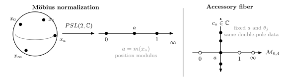
The position modulus $a\in\mathcal M_{0,4}$ labels the four-punctured sphere. With the local exponent differences fixed, $c_a$ moves along the one-dimensional affine fiber of projective connections above that point. The axes are schematic: both coordinates are complex, and the drawing does not assume $0<a<1$.

This picture is kinematic. Holding $c_a$ fixed while $a$ moves generally changes holonomy, while one scalar monodromy or spectral condition may select nonlinear branches $c_a(a)$.

Why Heun alone is not an isomonodromic family

Fixing the full four-point monodromy belongs naturally to a rank-two Fuchsian system. Its scalar reduction generically introduces a moving apparent singularity, so pure Heun equations occur only on special slices of that problem. Chapter 5 develops this distinction.

What the accessory coefficient controls

For a nonresonant normal-form singularity with exponent difference $\theta_j$, the local powers are

$$(z-z_j)^{(1\pm\theta_j)/2}.$$

The lift naturally induced by these normal-form powers has eigenvalues

$$-\ee^{\pm\pi\ii\theta_j}$$

and trace

$$\operatorname{tr}M_j = -2\cos(\pi\theta_j).$$

These local conjugacy data depend on $\theta_j$, not on $c_a$. By contrast, relative data such as

$$\operatorname{tr}(M_0M_1), \qquad \operatorname{tr}(M_1M_a), \qquad \operatorname{tr}(M_aM_0)$$

are global and generally vary with the accessory coefficient.

With the ordered relation

$$M_0M_aM_1M_\infty=I,$$

the generic fixed-local-class character variety is a complex surface. At fixed $a$, the one-dimensional accessory line generically maps by holonomy to a curve on that surface. Allowing both $a$ and $c_a$ to vary gives a two-dimensional coefficient family. This dimension match does not imply that the holonomy map is globally one-to-one or onto.

Resonance can expose the accessory locally

The simple-pole residue never enters the indicial equation, but at an integer exponent difference it can enter the later compatibility condition that decides whether a logarithm occurs. A concrete Heun family makes this visible. Take

$$a=2, \qquad \alpha=\beta=1, \qquad \gamma=\delta=2, \qquad \epsilon=-1.$$

The Fuchs relation holds, and

$$\begin{aligned} y'' &+ \left( \frac2z+\frac2{z-1}-\frac1{z-2} \right)y'\\ &+ \frac{z-q}{z(z-1)(z-2)}y =0. \end{aligned}$$

At $z=2$ the exponents are $0$ and $2$. Put $t=z-2$. The two coefficient functions have expansions

$$p(t) = -\frac1t+3+O(t)$$

and

$$r(t) = \frac{2-q}{2t} + \frac{3q-4}{4} + O(t).$$

For $y=b_0+b_1t+b_2t^2+\cdots$, the coefficient of $t^{-1}$ gives

$$b_1=\frac{2-q}{2}b_0.$$

At the resonant step the $b_2$ terms cancel. The remaining compatibility condition is

$$\frac{(q-3)(q-4)}4\,b_0=0.$$

Therefore $q=3$ and $q=4$ make the puncture apparent: both standard-form solutions are holomorphic and its local monodromy is $I$. For every other $q$, a logarithm occurs and the local monodromy has a nontrivial unipotent part.

The same conclusion in normal-form coordinates is especially instructive:

$$\begin{gathered} \left( \Delta_0,\Delta_1,\Delta_a,\Delta_\infty \right) = \left( 0,0,-\frac34,\frac14 \right),\\ \Lambda=1, \qquad \kappa_{\mathrm H}=q-3, \qquad c_a=\frac{5-q}{2}. \end{gathered}$$

Apparency occurs at $c_a=1$ or $c_a=1/2$. By contrast, $c_a=0$ occurs at $q=5$ and is not apparent. The puncture is not ordinary either: its double pole remains. In the normal determinant-one lift the log-free local monodromy is $-I$; the Liouville gauge converts it to $I$ in standard form, and both are projectively trivial.

Datum	What fixes it?
Marked-sphere geometry	The cross-ratio $a$, up to relabeling
Local monodromy eigenvalues	The exponent differences $\theta_j$
Resonant logarithm or apparency	A compatibility condition that can involve the accessory coordinate
Scalar differential equation with those data	One accessory coordinate, such as $c_a$ or $q$
Global monodromy representation	Analytic continuation of that equation
Distinguished or spectral accessory values	Additional monodromy, regularity, apparency, or boundary conditions

Here $c_a$ labels the full affine family of projective connections with the stated polar data. In the uniformization literature, “the accessory parameter problem” often means selecting the special value whose projective monodromy is Fuchsian. Isomonodromic, conformal-block, and spectral problems impose different global selection rules, developed in later chapters.

The accessory parameter is therefore not “the monodromy.” It is a coefficient coordinate whose dependence on monodromy is nonlinear; an inverse monodromy problem may also have several branches. At resonance, the exponent difference fixes the eigenvalues but not by itself the logarithmic or Jordan data.

Common pitfalls

Confusing the base with the fiber. The cross-ratio $a$ moves a puncture; $c_a$ changes the equation while the punctures stay fixed. Both are global data, but they answer different questions.

Calling zero accessory canonical. The equation $c_a=0$ depends on the chosen coordinate and reference projective connection. It neither removes the fourth puncture nor implies trivial monodromy.

Calling an apparent point ordinary. In this book, an apparent point has two holomorphic scalar solutions and local monodromy $I$ in the stated standard-form gauge. After the multivalued Liouville gauge, the natural normal-form lift may instead be $-I$; its projective monodromy is still trivial. An ordinary point additionally requires the coefficient poles to disappear in the chosen scalar gauge.

Forgetting that punctures are labeled. The six anharmonic values describe one generic unlabeled configuration, but exponent and basis labels must be permuted with the points.

Using the wrong number of constraints at infinity. A marked regular singularity at infinity imposes two conditions on the finite residues. An ordinary infinity imposes three.

Equating local traces with global monodromy. Fixed local exponents fix individual conjugacy classes only in the nonresonant generic setting. Products of monodromy matrices and connection data still depend on the accessory coefficient.

Exercises

1. Normalize an ordered quadruple

Verify that

$$m(z) = \frac{ (z-x_0)(x_1-x_\infty) }{ (z-x_\infty)(x_1-x_0) }$$

sends $(x_0,x_1,x_\infty)$ to $(0,1,\infty)$. Compute $a=m(x_a)$ for

$$(x_0,x_1,x_a,x_\infty)=(0,2,3,\infty).$$

Solution

Substitution gives $m(x_0)=0$. At $z=x_1$, numerator and denominator are the same product, so $m(x_1)=1$. The denominator vanishes at $x_\infty$, while the numerator is nonzero because the points are distinct, so $m(x_\infty)=\infty$.

When $x_\infty=\infty$, divide the factors involving $x_\infty$ before taking the limit:

$$\lim_{x_\infty\to\infty} \frac{x_1-x_\infty}{z-x_\infty} =1.$$

Therefore the example has

$$m(z)=\frac z2, \qquad a=m(3)=\frac32.$$

2. Count and reconstruct the accessory residues

For $n\geq3$ regular singularities with $n-1$ finite positions, expand the normal-form coefficient at infinity and count the free residues. Then specialize to $0$, $1$, $a$, and $\infty$, solve for $c_0,c_1$ in terms of $c_a$, and recover the compact simple-pole term.

Solution

Use

$$\frac1{z-z_j} = \frac1z+\frac{z_j}{z^2}+O(z^{-3})$$

and

$$\frac1{(z-z_j)^2} = \frac1{z^2}+O(z^{-3}).$$

Then

$$\begin{aligned} T(z) &= \frac1z\sum_jc_j\\ &\quad+ \frac1{z^2} \sum_j \left( \Delta_j+z_jc_j \right) + O(z^{-3}). \end{aligned}$$

Prescribing a regular singularity at infinity gives

$$\sum_jc_j=0, \qquad \sum_j \left( \Delta_j+z_jc_j \right) = \Delta_\infty.$$

Thus $n-1$ residues obey two independent constraints, leaving $n-3$. For finite positions $0,1,a$, these equations become

$$c_0+c_1+c_a=0$$

and

$$c_1+ac_a = \Delta_\infty-\Delta_0-\Delta_1-\Delta_a = \Lambda.$$

Therefore

$$c_1=\Lambda-ac_a, \qquad c_0=-\Lambda+(a-1)c_a.$$

Finally,

$$\begin{aligned} \frac{c_0}{z} + \frac{c_1}{z-1} + \frac{c_a}{z-a} &= \frac{\Lambda}{z(z-1)}\\ &\quad+ \frac{a(a-1)c_a}{z(z-1)(z-a)}. \end{aligned}$$

3. Audit the three accessory coordinates

At fixed $a$ and exponent data, start from

$$c_a = \frac{a\Lambda-\kappa_{\mathrm H}}{a(a-1)}, \qquad \kappa_{\mathrm H} = q-\frac{\gamma}{2}(a\delta+\epsilon).$$

Derive $\partial c_a/\partial q$, reconstruct $q$ from $c_a$, and compute $\partial T/\partial q$.

Solution

Only $\kappa_{\mathrm H}$ depends on $q$, with unit derivative. Hence

$$\frac{\partial c_a}{\partial q} = -\frac1{a(a-1)}.$$

Solving the affine relation for $q$ gives

$$q = \frac{\gamma}{2} \left( a\delta+\epsilon \right) + a\Lambda-a(a-1)c_a.$$

The $q$-dependent part of the normal coefficient is

$$T(z) \supset \frac{-\kappa_{\mathrm H}}{z(z-1)(z-a)}.$$

Therefore

$$\frac{\partial T}{\partial q} = -\frac1{z(z-1)(z-a)}.$$

This derivative is invariant under exponent-dependent affine shifts of the chosen accessory origin, but its normalization still depends on the coordinate convention.

4. Recover the local monodromy lift

Starting from the two normal-form powers

$$(z-z_j)^{(1\pm\theta_j)/2},$$

derive the eigenvalues and trace of the determinant-one local monodromy lift. Explain why nonintegral $\theta_j$ fixes its semisimple conjugacy class, whereas integral $\theta_j$ does not determine the logarithmic Jordan part.

Solution

One counterclockwise turn multiplies the two powers by

$$\exp \left[ 2\pi\ii\frac{1\pm\theta_j}{2} \right] = -\ee^{\pm\pi\ii\theta_j}.$$

Their product is one, so this is a determinant-one lift. Its trace is

$$\operatorname{tr}M_j = -2\cos(\pi\theta_j).$$

If $\theta_j\notin\mathbb Z$, the eigenvalues are distinct, so they determine a semisimple $SL(2,\mathbb C)$ conjugacy class. If $\theta_j\in\mathbb Z$, the eigenvalues coincide. A log-free basis gives $M_j=\pm I$ in this lift, whereas a logarithmic solution gives a nontrivial Jordan matrix with the same trace. The exponent difference alone cannot distinguish these cases.

5. Derive the resonant no-log condition

In the general Heun equation, set $\epsilon=-1$ and define

$$A=a\alpha\beta-q.$$

Put $t=z-a$ and $y=b_0+b_1t+b_2t^2+\cdots$. Show that the no-log compatibility condition at the exponent difference $2$ is

$$\begin{aligned} 0 ={}& A^2\\ &+ \left[ \gamma(a-1)+\delta a-(2a-1) \right]A\\ &+ \alpha\beta a(a-1). \end{aligned}$$

Then recover the apparent values for $a=2$, $\alpha=\beta=1$, and $\gamma=\delta=2$.

Solution

Write

$$D_0=a(a-1), \qquad D_1=2a-1.$$

The coefficient functions have the local expansions

$$p(t) = -\frac1t + \left( \frac\gamma a+\frac\delta{a-1} \right) + O(t)$$

and

$$r(t) = \frac{A}{D_0t} + \frac{\alpha\beta}{D_0} - \frac{AD_1}{D_0^2} + O(t).$$

The coefficient of $t^{-1}$ in the differential equation gives

$$-b_1+\frac{A}{D_0}b_0=0,$$

so $b_1=Ab_0/D_0$. At order $t^0$, the two contributions containing $b_2$ cancel. Dividing by $b_0$ and multiplying by $D_0^2$ gives

$$\begin{aligned} 0 ={}& A^2\\ &+ \left[ \gamma(a-1)+\delta a-D_1 \right]A\\ &+ \alpha\beta D_0, \end{aligned}$$

which is the required condition. For the stated specialization, $A=2-q$, $D_0=2$, and the coefficient of $A$ is $3$. Hence

$$(2-q)^2+3(2-q)+2 = (q-3)(q-4) =0.$$

Thus $q=3$ and $q=4$ are exactly the apparent values. In either case the smaller-exponent solution is holomorphic, and the larger-exponent Frobenius solution is already holomorphic.

6. Separate three special loci

For the same resonant family, compare:

1. the apparent values;
2. the value at which $c_a=0$;
3. the condition for the pole at $z=a$ to disappear from the standard Heun equation.

Explain why these are different notions.

Solution

For this family,

$$c_a=\frac{5-q}{2}.$$

The apparent values $q=3$ and $q=4$ therefore correspond to

$$c_a=1 \qquad\text{and}\qquad c_a=\frac12.$$

By contrast, $c_a=0$ occurs at $q=5$. The resonant obstruction there is

$$\frac{(5-3)(5-4)}4=\frac12\ne0,$$

so a logarithm is present.

For a general Heun equation, removing the pole at $z=a$ from the standard-form coefficients requires both

$$\epsilon=0 \qquad\text{and}\qquad q=a\alpha\beta.$$

The present family has $\epsilon=-1$, so the pole never disappears. In the book’s standard-form convention, apparency means two holomorphic scalar solutions and local monodromy $I$ even though coefficient poles may remain. The equation $c_a=0$ merely removes one simple-pole residue in a chosen normal-form decomposition; an ordinary point requires the coefficient poles themselves to vanish.

7. Recover the geometric dimension

Let $\mathscr D$ be the divisor of $n\geq3$ distinct points on $\mathbb P^1$. Use the genus-zero Riemann–Roch formula to compute

$$\dim H^0 \left( \mathbb P^1, K_{\mathbb P^1}^{\otimes2}(\mathscr D) \right).$$

For $n=4$, verify directly that $\omega_a$ has at most simple poles at all four punctures.

Solution

On $\mathbb P^1$,

$$\deg K_{\mathbb P^1}=-2.$$

Therefore

$$\deg \left[ K_{\mathbb P^1}^{\otimes2}(\mathscr D) \right] = -4+n.$$

For a line bundle of degree $d$ on $\mathbb P^1$,

$$h^0=\max\{d+1,0\}.$$

Hence, for $n\geq3$,

$$h^0=n-3.$$

For four points,

$$\omega_a = \frac{ a(a-1)\,dz^2 }{ z(z-1)(z-a) }$$

plainly has simple finite poles at $0$, $1$, and $a$. Near infinity, set $w=1/z$. Since $dz^2=w^{-4}dw^2$ and the rational coefficient is $a(a-1)z^{-3}+O(z^{-4})$, one obtains

$$\omega_a = \left[ \frac{a(a-1)}w+O(1) \right]dw^2.$$

Thus infinity is also only a simple pole. The one-dimensional space is spanned by $\omega_a$.

References

• NIST Digital Library of Mathematical Functions, §1.13(iv) gives the Liouville–Schwarzian coordinate law; §31.14(i), equations 31.14.1–31.14.5, gives the general second-order Fuchsian equation and its accessory-parameter count; and §31.2(i)–(ii), equations 31.2.1–31.2.4, identifies $a$ and $q$ as the singularity and accessory parameters of the general Heun equation.
• F. C. S. Brown, “Multiple zeta values and periods of moduli spaces $\mathcal M_{0,n}$”, Annales scientifiques de l’École Normale Supérieure 42 (2009), 371–489, §2.1, pp. 381–382, equations (2.1)–(2.3), defines labeled pointed-sphere moduli, cross-ratio coordinates, and the effective anharmonic action.
• R. S. Maier, “The 192 solutions of the Heun equation”, Mathematics of Computation 76 (2007), 811–843, Introduction and §2, equations (2.1)–(2.3), and §3, gives the $n-3$ accessory count and the Heun cross-ratio orbit in a normalized Fuchsian convention.
• K. Iwasaki, H. Kimura, S. Shimomura, and M. Yoshida, From Gauss to Painlevé: A Modern Theory of Special Functions, Vieweg, 1991, develops Fuchsian equations, monodromy, and deformation geometry from the rigid hypergeometric case onward.
• H. M. Farkas and I. Kra, Riemann Surfaces, 2nd ed., Springer, 1992, supplies the Möbius, cross-ratio, divisor, and Riemann–Roch background used here.
• L. A. Takhtajan and P. G. Zograf, “Hyperbolic 2-spheres with conical singularities, accessory parameters and Kähler metrics on $\mathcal M_{0,n}$”, Transactions of the American Mathematical Society 355 (2003), 1857–1867, Lemma 1, equations (5)–(7), relates Fuchsian accessory parameters to pointed-sphere moduli. Its equation uses $u''+\tfrac12T_\varphi u=0$, so its printed residues differ by a factor of two from this page’s convention.
• A. Ronveaux (ed.), Heun’s Differential Equations, Oxford University Press, 1995, Part A, records the canonical Heun equation, its transformations, and accessory-parameter conventions.