Connection Matrices and Wronskian Identities

A connection matrix compares two normalized solution frames after they have been continued to the same branch. For a second-order scalar equation, every entry is a Wronskian ratio. That elementary observation supplies a complete audit system: it fixes signs and directions, proves constancy, detects degenerate bases, and turns boundary conditions into zeros of specified matrix entries.

Throughout this page,

$$\Wr[f,g]=fg'-f'g, \qquad \Phi_\beta=\Phi_\alpha C_{\alpha\beta}.$$

The path, branches, and ordered bases are part of the symbol $C_{\alpha\beta}$ even when they are suppressed typographically.

Connection data form a groupoid

Let $\Phi_\alpha,\Phi_\beta,\Phi_\gamma$ be normalized fundamental matrices continued onto one simply connected overlap. Since any two fundamental matrices of the same system differ on the right by a constant,

$$\Phi_\beta=\Phi_\alpha C_{\alpha\beta}, \qquad C_{\alpha\beta}\in GL(n,\mathbb C).$$

The direction in the subscripts labels the frame transition $\alpha\to\beta$: the columns of $C_{\alpha\beta}$ are the $\alpha$-frame coordinates of the $\beta$ basis vectors. Equivalently, if one fixed solution has coefficient columns $v_\alpha$ and $v_\beta$, then

$$v_\alpha=C_{\alpha\beta}v_\beta.$$

Thus the induced coordinate map runs from $\beta$-coordinates to $\alpha$-coordinates. For the compatible reversed path and branch,

$$C_{\alpha\alpha}=I, \qquad C_{\beta\alpha}=C_{\alpha\beta}^{-1},$$

and

$$C_{\alpha\gamma} = C_{\alpha\beta}C_{\beta\gamma}.$$

The last identity follows directly:

$$\Phi_\gamma = \Phi_\beta C_{\beta\gamma} = \Phi_\alpha C_{\alpha\beta}C_{\beta\gamma}.$$

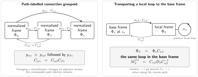
Connection data as a path-labelled groupoid. Compatible transitions satisfy $C_{\alpha\gamma}=C_{\alpha\beta}C_{\beta\gamma}$, while a local loop $D_\beta$ becomes $C_{*\beta}D_\beta C_{*\beta}^{-1}$ in the base frame.

Two related structures share this multiplication law. Fixed single-valued flat frames on an open cover give locally constant transition matrices on connected overlaps; on compatible triple overlaps they form a Čech cocycle. Homotopy classes of continuation paths, by contrast, are the arrows of the fundamental path groupoid. Choosing a frame at each endpoint turns analytic continuation into a frame-dependent representation of that groupoid by matrices.

The overlap cocycle and the continuation groupoid should not be conflated, even though both lead to the displayed product. A path-labelled connection matrix without its endpoints, path class, and chosen frames is not an invariant number.

Independent changes of local basis

Let

$$\widetilde\Phi_\alpha=\Phi_\alpha H_\alpha, \qquad \widetilde\Phi_\beta=\Phi_\beta H_\beta.$$

Then

$$\widetilde C_{\alpha\beta} = H_\alpha^{-1} C_{\alpha\beta} H_\beta.$$

This two-sided covariance is more general than monodromy conjugation. The same matrix $H$ acts at both ends only when one global base frame is changed. Changing the leading coefficient of one Frobenius vector, the normalization of one Jost solution, or the lateral sum at one end produces genuinely independent factors.

Paths insert monodromy

Suppose a path change replaces the continued frames on the common branch by

$$\Phi_\alpha M_\alpha, \qquad \Phi_\beta M_\beta.$$

The new connection matrix is

$$C_{\alpha\beta}^{\mathrm{new}} = M_\alpha^{-1} C_{\alpha\beta} M_\beta.$$

This is the safest way to handle a path winding around a puncture: determine which endpoint frame acquired which monodromy, then use the basis-covariance law. Guessing whether to multiply a connection coefficient “on the left or right” is unnecessary.

Four Wronskians recover four entries

For one scalar second-order equation, write

$$\Phi_\alpha=(f_1,f_2), \qquad \Phi_\beta=(g_1,g_2),$$

where the notation includes the derivative row. Let

$$C_{\alpha\beta} = \begin{pmatrix} c_{11}&c_{12}\\ c_{21}&c_{22} \end{pmatrix}.$$

The first column of $\Phi_\beta=\Phi_\alpha C_{\alpha\beta}$ says

$$g_1=c_{11}f_1+c_{21}f_2.$$

Taking Wronskians with $f_2$ and $f_1$ gives

$$c_{11} = \frac{\Wr[g_1,f_2]}{\Wr[f_1,f_2]}, \qquad c_{21} = \frac{\Wr[f_1,g_1]}{\Wr[f_1,f_2]}.$$

The second column gives the full formula

$$C_{\alpha\beta} = \frac1{\Wr[f_1,f_2]} \begin{pmatrix} \Wr[g_1,f_2]&\Wr[g_2,f_2]\\ \Wr[f_1,g_1]&\Wr[f_1,g_2] \end{pmatrix}.$$

Every sign follows from the declared order in $\Wr[f,g]$. Swapping the Wronskian convention or the basis columns changes the printed matrix.

Why the ratios are constant

For

$$y''+p(z)y'+q(z)y=0,$$

every Wronskian of two solutions satisfies

$$\Wr'=-p\,\Wr.$$

All four numerators and the denominator therefore carry the same Abel factor. Their ratios are constant on the chosen branch, even when the individual Wronskians are not. In Liouville normal form $p=0$, each Wronskian is itself constant.

The hypothesis “solutions of the same equation on the same branch” matters. A common dependent-variable gauge or coordinate change applied to both bases multiplies all relevant Wronskians by the same nonzero factor, so the ratios remain unchanged. Trouble arises when numerator and denominator are formed in different gauges or coordinates, or from solutions at different spectral parameters.

Determinants and the Plücker check

Taking determinants of $\Phi_\beta=\Phi_\alpha C_{\alpha\beta}$ gives

$$\det C_{\alpha\beta} = \frac{\Wr[g_1,g_2]}{\Wr[f_1,f_2]}.$$

This is usually the quickest exact check of a complicated gamma-function or asymptotic connection matrix. It also explains why $\det C_{\alpha\beta}=1$ is not automatic: it requires compatible Wronskian normalizations at both ends.

The four-entry formula and determinant identity are related by the two-dimensional Plücker relation:

$$\begin{aligned} &\Wr[f,g]\Wr[h,k] -\Wr[f,h]\Wr[g,k]\\ &\qquad +\Wr[f,k]\Wr[g,h] =0. \end{aligned}$$

It is simply the alternating determinant identity for four vectors in a two-dimensional solution space. Applied to $f_1,f_2,g_1,g_2$, it reduces the determinant of the reconstructed matrix to the Wronskian ratio above.

For an $n\times n$ system the universal formula is

$$C_{\alpha\beta} = \Phi_\alpha^{-1}\Phi_\beta.$$

The determinant ratio remains valid. Individual entries are obtained from cofactors or exterior-power minors rather than scalar two-function Wronskians.

Local monodromy in a transported frame

Let $\Phi_i$ be a local normalized frame and $\Phi_*$ a base frame continued along a declared path, with

$$\Phi_i=\Phi_*C_{*i}.$$

If a positive local loop acts by

$$\Phi_i^\gamma=\Phi_iD_i,$$

then the same based loop in the base frame has

$$M_i^{(*)} = C_{*i}D_iC_{*i}^{-1}.$$

For an irregular point, replace $D_i$ by the complete actual local product

$$M_{\mathrm{loc},i} = M_{\mathrm f,i} S_{i,m-1}^{-1}\cdots S_{i,0}^{-1}.$$

A raw Stokes factor connects two sector frames and is not automatically conjugated by one common $C_{*i}$; it first needs sector-specific transport to a common tangential frame. The wild-monodromy page keeps that distinction explicit.

Boundary coefficients are connection entries

Let

$$\Phi_L=(u_L,v_L), \qquad \Phi_R=(u_R,v_R),$$

and suppose

$$\Phi_R=\Phi_LC_{LR}.$$

The first right-normalized solution has the expansion

$$u_R = (C_{LR})_{11}u_L +(C_{LR})_{21}v_L.$$

Consequently,

$$\Wr[u_L,u_R] = (C_{LR})_{21} \Wr[u_L,v_L].$$

If $u_L$ and $u_R$ are the solutions selected by the left and right boundary conditions, they are proportional exactly when

$$\Wr[u_L,u_R]=0,$$

or, for a nondegenerate left basis,

$$(C_{LR})_{21}=0.$$

The Wronskian may be evaluated at any interior regular matching point. For

$$y''+p(x,\lambda)y'+q(x,\lambda)y=0,$$

the raw value depends on that point when $p\ne0$, but its zero set does not. On a fixed integration path, the Abel-normalized boundary function

$$\begin{aligned} D(\lambda) &= \exp\left( \int_{x_0}^{x}p(s,\lambda)\,\dd s \right)\\ &\qquad{}\times \Wr[u_L,u_R](x,\lambda) \end{aligned}$$

is independent of $x$. Under $u_L\mapsto a(\lambda)u_L$ and $u_R\mapsto b(\lambda)u_R$, it changes by $D\mapsto abD$. Analytic nowhere-zero factors preserve its zeros and their multiplicities; zeros or poles in the normalizing factors need not.

This is the algebraic bridge from a connection problem to a boundary or spectral condition. The particular vanishing entry changes if either basis is reordered. Match-point independence alone does not make $D$ a canonical spectral determinant. Later pages add the analytic hypotheses needed to call it a Jost function, an Evans function, or one of several inequivalent determinant constructions.

An elementary shifted-basis benchmark

Consider

$$y''+k^2y=0$$

and the initial-value frames normalized at $0$ and $L$:

$$\Phi_0(z) = \begin{pmatrix} \cos(kz)&\dfrac{\sin(kz)}k\\ -k\sin(kz)&\cos(kz) \end{pmatrix},$$ $$\Phi_L(z) = \begin{pmatrix} \cos(k(z-L))& \dfrac{\sin(k(z-L))}k\\ -k\sin(k(z-L))& \cos(k(z-L)) \end{pmatrix}.$$

Both have determinant one. Since $\Phi_0(0)=I$,

$$\Phi_L=\Phi_0C_{0L},$$

with

$$C_{0L} = \begin{pmatrix} \cos(kL)&-\dfrac{\sin(kL)}k\\ k\sin(kL)&\cos(kL) \end{pmatrix}.$$

The determinant identity is the trigonometric relation

$$\cos^2(kL)+\sin^2(kL)=1.$$

For a second shift $M$,

$$C_{0,L+M} = C_{0L}C_{L,L+M},$$

which is exactly the sine and cosine addition law. The apparent factors $1/k$ are removable:

$$\lim_{k\to0}C_{0L} = \begin{pmatrix} 1&-L\\ 0&1 \end{pmatrix}.$$

This limit is the connection matrix between the shifted initial-value bases of $y''=0$. A well-normalized basis makes the parameter limit regular before any special-function simplification.

Resonance and normalization failures

The Wronskian denominator vanishes when the displayed “basis” loses rank. That can happen even though the differential equation and its solution local system remain regular in the parameter.

For a resonant Frobenius family, make a suitable parameter-dependent linear recombination—often a divided difference—while holding the logarithm branch fixed, then verify that the finite limit solves the limiting homogeneous equation. A bare parameter derivative is not a universal remedy: if $L_\nu y_\nu=0$, then

$$L_{\nu_0} \left. \partial_\nu y_\nu \right|_{\nu_0} = - \left. (\partial_\nu L_\nu)y_\nu \right|_{\nu_0},$$

which is generally inhomogeneous. Resonance permits a logarithmic solution but does not force one; its logarithmic coefficient can vanish. The Euler family is especially simple because the operator’s first derivative in $\nu$ vanishes at $\nu=0$:

$$z^2y''+zy'-\nu^2y=0.$$

On a fixed branch of $\log z$, the basis $(z^\nu,z^{-\nu})$ collapses at $\nu=0$. The recombination

$$\begin{aligned} u_\nu &= \frac{z^\nu+z^{-\nu}}2,\\ v_\nu &= \frac{z^\nu-z^{-\nu}}{2\nu} \end{aligned}$$

has the regular limit

$$(u_0,v_0) = \left( 1,\log z \right)$$

and

$$\Wr[u_\nu,v_\nu]=\frac1z.$$

Individual entries of a connection matrix may therefore have poles because the chosen local normalization degenerates. If

$$\widetilde\Phi_\alpha = \Phi_\alpha B_\alpha(\nu), \qquad \widetilde\Phi_\beta = \Phi_\beta B_\beta(\nu),$$

then

$$\widetilde C_{\alpha\beta} = B_\alpha(\nu)^{-1} C_{\alpha\beta} B_\beta(\nu).$$

The matrices $B_\alpha,B_\beta$ may be singular at the limiting parameter provided they are invertible away from it. If both recombined frames extend to nondegenerate limiting fundamental matrices—equivalently, their limiting Wronskians are nonzero—then a finite, invertible limit of $\widetilde C_{\alpha\beta}$ diagnoses a removable basis artifact. A finite but singular matrix accompanied by a collapsed frame does not. Failure of one proposed recombination is not decisive, although persistent failure can reflect a genuinely singular or degenerate parameter family.

Numerically, a different problem appears when one solution is exponentially dominant. Two large nearly parallel columns can make direct Wronskians lose relative precision. Scaled sectorial bases, logarithmic derivatives, exterior products, or matching near a balanced point improve conditioning without changing the exact identities.

A connection audit

For every substantial connection formula, check in this order:

1. write $\Phi_\beta=\Phi_\alpha C_{\alpha\beta}$ beside the matrix;
2. declare the ordered bases, branches, continuation path, and excluded parameters;
3. verify one column from leading behavior or a local value;
4. verify $\det C$ from the Wronskian ratio;
5. test $C_{\beta\alpha}=C_{\alpha\beta}^{-1}$ on the compatible reversed path and branch;
6. if a third frame is available, test the cocycle;
7. take a resonant, confluent, or elementary limit in recombined bases;
8. only then interpret a matrix entry as a boundary coefficient.

These checks are independent enough that a convention error rarely survives all of them.

Common pitfalls

Reversing the connection direction. The equation $\Phi_\beta=\Phi_\alpha C_{\alpha\beta}$ is part of the formula. Inverting a correct matrix without reversing its subscripts creates a wrong result.

Assuming every relevant Wronskian is constant. It is constant only when the first-derivative coefficient vanishes. For a general scalar equation, Wronskian ratios are constant because the Abel factors cancel.

Suppressing the continuation path. A different path can insert monodromy at either endpoint. Two sources can print different correct matrices for different path classes.

Calling a pole in an entry a singular connection problem. First test whether the local basis collapsed at resonance or its leading normalization vanished. Recombination can remove a basis artifact.

Reading the wrong boundary entry. The selected coefficient depends on which solution is the first column at each end. Derive it once from a Wronskian instead of relying on memory.

Exercises

1. Reconstruct the matrix. Starting only from $g_j=c_{1j}f_1+c_{2j}f_2$, derive all four Wronskian formulas and the determinant ratio.

Solution

For each $j$,

$$\Wr[g_j,f_2] = c_{1j}\Wr[f_1,f_2],$$

and

$$\Wr[f_1,g_j] = c_{2j}\Wr[f_1,f_2].$$

These identities give the two entries in column $j$. Since $\Phi_\beta=\Phi_\alpha C_{\alpha\beta}$,

$$\Wr[g_1,g_2] = \Wr[f_1,f_2]\det C_{\alpha\beta},$$

which proves the determinant formula.

2. Prove covariance and the cocycle. Derive the connection matrix after independent changes $H_\alpha,H_\beta$, then show that three compatible frames obey $C_{\alpha\gamma}=C_{\alpha\beta}C_{\beta\gamma}$.

Solution

From

$$\Phi_\beta H_\beta = \Phi_\alpha H_\alpha \widetilde C_{\alpha\beta}$$

and $\Phi_\beta=\Phi_\alpha C_{\alpha\beta}$, cancellation gives

$$\widetilde C_{\alpha\beta} = H_\alpha^{-1} C_{\alpha\beta} H_\beta.$$

Also,

$$\Phi_\gamma = \Phi_\beta C_{\beta\gamma} = \Phi_\alpha C_{\alpha\beta}C_{\beta\gamma}.$$

Uniqueness of the constant right factor gives the cocycle.

3. Verify the shifted oscillator. Derive $C_{0L}$ from the values at $z=0$, prove its determinant is one, and show that the cocycle is equivalent to the addition formulas.

Solution

Because $\Phi_0(0)=I$,

$$C_{0L}=\Phi_L(0),$$

which gives the displayed matrix. Its determinant is

$$\cos^2(kL)+\sin^2(kL)=1.$$

Multiplying the matrices for lengths $L$ and $M$ yields

$$\begin{aligned} \cos(k(L+M)) &= \cos(kL)\cos(kM) -\sin(kL)\sin(kM),\\ \sin(k(L+M)) &= \sin(kL)\cos(kM) +\cos(kL)\sin(kM). \end{aligned}$$

These are precisely the entries required by $C_{0,L+M}=C_{0L}C_{L,L+M}$.

4. Locate a boundary coefficient. With $\Phi_R=\Phi_LC_{LR}$, prove that proportionality of $u_L$ and $u_R$ is the condition $(C_{LR})_{21}=0$.

Solution

The first column gives

$$u_R = (C_{LR})_{11}u_L +(C_{LR})_{21}v_L.$$

Taking the Wronskian with $u_L$ gives

$$\Wr[u_L,u_R] = (C_{LR})_{21} \Wr[u_L,v_L].$$

Since $\Phi_L$ is a fundamental matrix, $\Wr[u_L,v_L]\ne0$. Thus $u_L,u_R$ are proportional exactly when $(C_{LR})_{21}=0$.

5. Recombine the Euler resonance. Prove the limit and Wronskian formulas for $(u_\nu,v_\nu)$. Then find its limiting positive monodromy.

Solution

Using

$$z^{\pm\nu} = \ee^{\pm\nu\log z} = 1\pm\nu\log z +O(\nu^2),$$

one finds

$$u_\nu\longrightarrow1, \qquad v_\nu\longrightarrow\log z.$$

Since

$$\Wr[z^\nu,z^{-\nu}] = -\frac{2\nu}{z},$$

and the recombination matrix has determinant $-1/(2\nu)$,

$$\Wr[u_\nu,v_\nu]=\frac1z.$$

Positive continuation of the limiting basis gives

$$\left( 1,\log z \right)^\gamma = \left( 1,\log z \right) \begin{pmatrix} 1&2\pi\ii\\ 0&1 \end{pmatrix}.$$

References

• NIST Digital Library of Mathematical Functions, §1.13, Differential Equations, for Abel’s identity and Wronskian conventions.
• NIST Digital Library of Mathematical Functions, §1.13(ii), Equations with a Parameter, for analytic dependence on parameters.
• NIST Digital Library of Mathematical Functions, §15.10(i–ii), Hypergeometric Differential Equation, for logarithmic resonant bases and connection formulas with their parameter restrictions.
• NIST Digital Library of Mathematical Functions, §13.2(vi–vii), Kummer Functions, for Wronskians, integer-parameter logarithmic solutions, and limiting conventions.
• K. Iwasaki, H. Kimura, S. Shimomura, and M. Yoshida, From Gauss to Painlevé: A Modern Theory of Special Functions, for connection problems, monodromy, and normalized special-function bases.
• Y. Haraoka, Linear Differential Equations in the Complex Domain, Springer, 2020, for monodromy and connection problems.
• E. L. Ince, Ordinary Differential Equations, Dover, 1956, for classical Wronskian and connection theory.
• F. W. J. Olver, Asymptotics and Special Functions, AKP Classics, 1997, for asymptotic bases, connection coefficients, and numerical conditioning.
• T. Kapitula and K. Promislow, Spectral and Dynamical Stability of Nonlinear Waves, Springer, 2013, for boundary-value Evans and Jost constructions.