Series, Fredholm Representations, and Numerical Realizations

An isomonodromic tau function can be computed without first solving the nonlinear Painlevé equation. Cut the punctured sphere into rigid three-point pieces, solve those pieces by hypergeometric functions, and measure whether their boundary data glue. The resulting obstruction is a Fredholm determinant:

$$\tau_{\mathrm J}(t;\mathcal M) = \Upsilon(t;\mathcal M) \det\!\left(I-\mathsf U(t;\mathcal M)\right).$$

Here $\mathcal M$ is fixed marked monodromy data, $\mathsf U$ is an auxiliary trace-class operator built from Riemann–Hilbert boundary projections, and $\Upsilon$ is explicit and nonzero on the chosen time chart. Writing $\mathsf U$ in Fourier modes gives a semi-infinite matrix; projecting its modes gives finite matrices, while expanding the exact Fourier matrix in principal minors gives an integer charge sum whose coefficients are labeled by pairs of partitions. Discretizing the contour instead gives a Nyström determinant. These are complementary realizations of the same isomonodromic object.

The adjective matters. The operator $I-\mathsf U$ glues an inverse Riemann–Hilbert problem; it is not the scalar differential operator whose eigenvalues, resonances, or quasinormal modes may be under study. This page therefore develops an exact determinant formula and a numerical laboratory while retaining the spectral firewall.

First pass

Read the object ledger, the four-pole gluing formula, and the finite-section algorithm. The charged-partition derivation explains where the series comes from; the trace-norm and Hamiltonian checks explain when a computed number should be trusted.

Five objects share dangerously similar names

The same calculation may contain all five objects below. The JMU function, the RH determinant, and the fully convergent principal-minor series are exactly equivalent on their shared chart. A finite section or truncated series is only an approximation.

Object	Definition	What a zero means
JMU tau function $\tau_{\mathrm J}$	A local potential of the JMU one-form, $\dd\log\tau_{\mathrm J}=\omega_{\mathrm{JMU}}$	A point of the Malgrange divisor after holomorphic continuation
RH Fredholm determinant $D_{\mathrm{RH}}=\det(I-\mathsf U)$	An ordinary Fredholm determinant of an auxiliary trace-class gluing operator	Failure of the normalized inverse RH problem, provided $\Upsilon\neq0$
Fourier or Nyström determinant $D_L^{\mathrm{Four}}$, $D_m^{\mathrm{Nys}}$	A determinant of a finite matrix approximating $\mathsf U$	A zero of a discretization; possibly a truncation artifact
Principal-minor series	A reorganization of $D_{\mathrm{RH}}$ by Fourier charge and partitions	The same exact divisor only after convergence and normalization have been established
Scalar spectral determinant $D_{\mathrm{sp}}(\lambda_{\mathrm{sp}})$	A boundary, resolvent, zeta, or Birman–Schwinger determinant for a declared scalar operator family	An eigenvalue, resonance, or QNM only on the declared operator domain and analytic sheet

An equality between the first two has the form

$$\tau_{\mathrm J} = \Upsilon D_{\mathrm{RH}}, \qquad \Upsilon\neq0.$$

It is therefore an equality of zero divisors on the chart. By contrast, $D_L^{\mathrm{Four}}\to D_{\mathrm{RH}}$ is a limiting statement. A few stable digits of $D_L^{\mathrm{Four}}$ are evidence, not an identity. An equality $D_{\mathrm{sp}}=g\tau_{\mathrm J}$ is a separate theorem that must identify the boundary lines and prove $g$ analytic and nowhere zero.

Ratios remove the arbitrary JMU constant

The definition on the JMU page fixes tau only up to $C(\mathcal M)\neq0$. Numerical comparisons should therefore favor

$$\mathcal R(t,t_*;\mathcal M) = \frac{\tau_{\mathrm J}(t;\mathcal M)} {\tau_{\mathrm J}(t_*;\mathcal M)}$$

and

$$H_t(t;\mathcal M) = \partial_t\log\tau_{\mathrm J}(t;\mathcal M).$$

Both are invariant under $\tau_{\mathrm J}\mapsto C(\mathcal M)\tau_{\mathrm J}$. The ratio still requires consistent analytic continuation: its numerator and denominator must use the same exponent lifts, logarithm branch, parametrix normalizations, and continuation paths.

A pants decomposition turns monodromy into an operator

Consider the traceless rank-two Fuchsian system

$$\frac{\dd Y}{\dd z} = \left( \frac{A_0}{z} + \frac{A_t}{z-t} + \frac{A_1}{z-1} \right)Y, \qquad A_\infty=-A_0-A_t-A_1.$$

The residue eigenvalues are $\pm\theta_\nu/2$. Fix the marked monodromy data and diagonalize the composite monodromy

$$M_{0t}=M_0M_t, \qquad \operatorname{tr}M_{0t} = 2\cos(\pi\sigma_{0t}).$$

Initially take $0<t<1$ and choose a counterclockwise circle $\mathcal C$ with

$$t<R<1, \qquad \mathcal C=\{z:|z|=R\}.$$

The circle separates $\{0,t\}$ from $\{1,\infty\}$. More generally one works on a simply connected complex time chart on which a homologous separating contour remains valid and no logarithm branch changes.

The cut produces two three-punctured spheres:

• the left trinion has singularities $\{0,t,\infty\}$ and composite exponent $\sigma_{0t}$ at its gluing boundary;
• the right trinion has singularities $\{0,1,\infty\}$ and the same gluing exponent.

After $z=t\zeta$ rescales the left trinion, both auxiliary systems have three singularities at $0,1,\infty$. A three-point rank-two Fuchsian system is rigid once its local and link data are fixed, so its entries are Gauss hypergeometric functions. This is the same rigidity used in the hypergeometric connection benchmark.

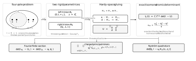
The separating circle turns the four-pole inverse problem into two rigid three-point parametrices. Their Hardy-space graph maps $\mathsf a$ and $\mathsf d$ form the off-diagonal gluing operator $\mathsf U$. The exact Fredholm determinant can then be approximated by Fourier finite sections or expanded into charged principal minors.

Plemelj graphs give the off-diagonal blocks

Let $\mathcal H_{\mathcal C}=\mathbb C^2\otimes L^2(\mathcal C)$ and split its Laurent modes into Hardy subspaces

$$\mathcal H_{\mathcal C} = \mathcal H_+\oplus\mathcal H_-.$$

The boundary values of each normalized three-point parametrix form the graph of an operator over the corresponding free Hardy subspace. Denote the two graph maps by

$$\mathsf a:\mathcal H_-\longrightarrow\mathcal H_+, \qquad \mathsf d:\mathcal H_+\longrightarrow\mathcal H_-.$$

Equivalently, they are differences of the dressed and free Plemelj projections. Their kernels are regular on the diagonal because the numerator vanishes when $z'=z$. The full gluing operator is

$$\mathsf U = \begin{pmatrix} 0&\mathsf a\\ \mathsf d&0 \end{pmatrix}.$$

Analyticity of the parametrices in a neighborhood of the separating annulus gives rapidly decaying Fourier coefficients and the trace-ideal properties needed by the ordinary Fredholm determinant. The block resolvent $(I-\mathsf U)^{-1}$ exists precisely when the two graph spaces can be glued to the normalized four-point solution.

Transpose the source convention before copying a kernel

The standard Fredholm construction used here is often printed for a row system $\partial_z\Phi=\Phi A$, with monodromy acting on the left. This book uses $\partial_zY=AY$ and right monodromy. One may set $\Phi=Y^{\mathsf T}$ inside the construction and transpose every product, or formulate the maps invariantly through Plemelj projections as above. Copying the printed matrix-kernel order without this translation generally produces the wrong operator.

The four-pole Fredholm formula fixes every factor of two

The literature convention behind the construction assigns residue eigenvalues $\pm\theta_{\nu,\mathrm{GL}}$ and composite eigenvalues $\exp(\pm2\pi\ii\sigma_{\mathrm{GL}})$. The present book assigns $\pm\theta_\nu/2$ and $\exp(\pm\pi\ii\sigma_{0t})$. Thus

$$\theta_{\nu,\mathrm{GL}} = \frac{\theta_\nu}{2}, \qquad \sigma_{\mathrm{GL}} = \frac{\sigma_{0t}}{2}.$$

In the book conventions the exact four-pole representation is

$$\boxed{ \tau_{\mathrm J}(t;\mathcal M) = C(\mathcal M)\, t^{\kappa_{0t}} \det\!\left(I-\mathsf U(t;\mathcal M)\right) },$$

where

$$\kappa_{0t} = \frac{ \sigma_{0t}^2-\theta_0^2-\theta_t^2 }{4}.$$

This is the page’s organizing identity. It is not a universal normalization convention: an explicit hypergeometric gauge can move a nowhere-zero elementary factor, such as a power of $1-t$, between the prefactor and the kernel. The invariant statement is

$$\tau_{\mathrm J} = \Upsilon\,\det(I-\mathsf U), \qquad \Upsilon\neq0$$

on the declared chart.

Branch and genericity data are part of the theorem

Choose $\Log t$ on the time chart and define

$$t^\alpha=\exp(\alpha\Log t).$$

Choose a lift of $\sigma_{0t}$ rather than only its trace cosine, and fix the twist coordinate $\eta_{\mathrm F}$ that completes the composite monodromy data. A convenient fundamental strip is

$$|\Re\sigma_{0t}|\leq1, \qquad \sigma_{0t}\neq0,\ \pm1.$$

For the simplest nonresonant hypergeometric formula, also avoid

$$\theta_0\pm\theta_t\pm\sigma_{0t}\in2\mathbb Z, \qquad \theta_1\pm\theta_\infty\pm\sigma_{0t}\in2\mathbb Z,$$

with all independent sign choices. These exclusions select a generic coordinate chart; they do not say that the tau function itself ceases to exist at every excluded value. At resonance, bases and individual coefficients can have poles while the complete expression has a finite logarithmic or limiting form.

The trace coordinate is invariant under $\sigma_{0t}\mapsto\pm\sigma_{0t}+2n$, but a particular series is not: changing the lift relabels its charge sectors and transforms the twist. Likewise, changing the normalization of either three-point parametrix can change $C(\mathcal M)$ and the coordinate used for $\eta_{\mathrm F}$ while leaving the JMU logarithmic derivative unchanged.

Fourier finite sections give a controlled small-time calculation

Use half-integer Fourier modes

$$z^{-1/2+p}, \qquad p\in\mathbb Z+\frac12.$$

The maps $\mathsf a$ and $\mathsf d$ connect opposite Hardy signs. After rescaling the left trinion, its matrix elements have the schematic form

$$\mathsf d^{-p}{}_{q}(t) = t^{-\mathfrak S} \widetilde{\mathsf d}^{-p}{}_{q} t^{\mathfrak S} t^{p+q}, \qquad p,q\in\mathbb Z_{\geq0}+\frac12,$$

where $\mathfrak S=\operatorname{diag} (\sigma_{0t}/2,-\sigma_{0t}/2)$ in a chosen composite eigenbasis. The coefficients of $\mathsf a$ and $\widetilde{\mathsf d}$ are time independent and follow from the two hypergeometric parametrices.

Two Fourier truncations answer different questions:

• for fixed $t$, the projection $\mathsf U_L^{\mathrm F}=P_L\mathsf U P_L$ retains the first $L$ positive modes and converges to the exact operator in trace norm;
• for the asymptotic expansion as $t\to0$, the degree-triangular truncation $\mathsf U_L^\triangle$ retains the coefficients with $p+q\leq L$ and sets the other entries of its first $L$ mode blocks to zero.

For rank two, the two nonzero blocks of $\mathsf U_L^\triangle$ are $2L\times2L$, and the full matrix is $4L\times4L$. The small-$t$ theorem gives

$$\tau_{\mathrm J}(t) = C\,t^{\kappa_{0t}} \left[ \det(I_{4L}-\mathsf U_L^\triangle) + O(t^L) \right]$$

in the generic fundamental strip. Under the strict condition $|\Re\sigma_{0t}|<1$, the bracketed remainder improves to $o(t^L)$. The estimate is a local asymptotic statement as $t\to0$; it is not a uniform certificate near $t=1$.

Finite block algebra halves the matrix size:

$$\begin{aligned} \det(I_{4L}-\mathsf U_L^\triangle) &= \det(I_{2L}-\mathsf a_L^\triangle\mathsf d_L^\triangle) \\ &= \det(I_{2L}-\mathsf d_L^\triangle\mathsf a_L^\triangle). \end{aligned}$$

The equality of the two reduced determinants is exact. Their disagreement in floating-point arithmetic is therefore a useful implementation test, but not an independent mathematical representation.

The first triangular section exposes three fractional branches

The $L=1$ degree-triangular section makes the branched structure visible without any partition notation. Normalize the right and rescaled left parametrices on the gluing annulus as

$$\begin{aligned} \Psi_R(z) &= \left(I+g_1^Rz+O(z^2)\right)G_R, \\ \Psi_L(z) &= t^{-\mathfrak S} \left( I+g_1^Lt z^{-1}+O(t^2z^{-2}) \right)G_L, \end{aligned}$$

$G_R$ and $G_L$ are constant frames. They cancel from the kernels through products of the form $\Psi(z)\Psi(z')^{-1}$. Every matrix power below uses the already fixed logarithm branch:

$$t^{\mathfrak S} = \exp\!\left(\mathfrak S\Log t\right).$$

Then, for $|\Re\sigma_{0t}|<1$,

$$\begin{aligned} \tau_{\mathrm J}(t) = C\,t^{\kappa_{0t}} \biggl\{ \det\left[ I-g_1^R t^{I-\mathfrak S} g_1^L t^{\mathfrak S} \right] + o(t) \biggr\}. \end{aligned}$$

Write $g_1^R=(r_{ij})$ and $g_1^L=(\ell_{ij})$. Direct expansion of the finite determinant gives

$$\begin{aligned} 1 &- r_{21}\ell_{12}t^{1-\sigma_{0t}} - \left( r_{11}\ell_{11} + r_{22}\ell_{22} \right)t \\ &- r_{12}\ell_{21}t^{1+\sigma_{0t}} + \det(g_1^R)\det(g_1^L)t^2. \end{aligned}$$

The powers $1-\sigma_{0t}$, $1$, and $1+\sigma_{0t}$ are the first fractional branches later reorganized by charge. The $t^2$ term is an exact algebraic check of this finite determinant; the $L=1$ theorem only controls the complete tau expression through $o(t)$.

Trace norm is the correct convergence test

For fixed $t$ on a compact subset of the chart, use the ordinary Fourier projection

$$\mathsf U_L^{\mathrm F} = P_L\mathsf U P_L$$

and suppose

$$\left\| \mathsf U-\mathsf U_L^{\mathrm F} \right\|_1 \longrightarrow0.$$

Then the determinant is continuous, with the standard bound

$$\begin{aligned} \left| \det(I-\mathsf U) - \det(I-\mathsf U_L^{\mathrm F}) \right| &\leq \|\mathsf U-\mathsf U_L^{\mathrm F}\|_1 \\ &\quad\times \exp\!\left( 1+\|\mathsf U\|_1+\|\mathsf U_L^{\mathrm F}\|_1 \right). \end{aligned}$$

Operator-norm convergence alone is insufficient for an ordinary Fredholm determinant. Nor does stabilization of the displayed digits bound the unseen tail. A proof-quality computation needs a trace-norm tail estimate, an equivalent coefficient majorant, or an interval enclosure of the omitted modes.

A stable Fourier workflow

1. Fix $\Log t$, the exponent lifts, the composite eigenbasis, and the twist normalization.
2. Generate the two three-point parametrices and their local coefficients independently; compare at one nonsingular point with direct hypergeometric evaluation.
3. Assemble each factor $t^{p+q+\sigma_\beta-\sigma_\alpha}$ as one exponential. Forming $t^{-\mathfrak S}$ and $t^{\mathfrak S}$ separately can create severe overflow and cancellation.
4. Compute $\log\det$ by pivoted LU or a rank-revealing factorization, recording both $\log|\det|$ and its complex phase. Near a zero, also monitor the smallest singular value of the relevant finite matrix $I-\mathsf U_L^{\mathrm F}$ or $I-\mathsf U_L^\triangle$.
5. Increase $L$ and precision separately. Varying both at once hides whether the dominant error is truncation, roundoff, or conditioning.
6. Repeat with a second contour radius $R$ inside the same annulus. The exact determinant is contour invariant after all associated normalizations are transported consistently.

Principal minors become charges and partitions

For a trace-class matrix in a Fourier basis, von Koch’s expansion reads

$$\det(I-\mathsf U) = \sum_{\mathfrak Y} \det(-\mathsf U)_{\mathfrak Y},$$

where $\mathfrak Y$ ranges over finite index subsets and the subscript denotes the corresponding principal minor. The off-diagonal block form forces a balance: a nonzero minor chooses the same total number of positive and negative Hardy modes.

For rank two, the selected modes can be read as particles and holes in two half-integer Maya diagrams. Each diagram is equivalent to a charged partition. The zero-total-charge condition leaves

$$(Y_+,n), \qquad (Y_-,-n), \qquad n\in\mathbb Z.$$

Thus the determinant has the local structure

$$\begin{aligned} \tau_{\mathrm J}(t) &= C \sum_{n\in\mathbb Z} s_{\mathrm F}^{\,n} \mathcal C_n(\boldsymbol\theta,\sigma_{0t}) t^{\kappa_n} \\ &\quad\times \sum_{Y_+,Y_-} \mathcal B_{Y_+,Y_-}^{(n)} (\boldsymbol\theta,\sigma_{0t}) t^{|Y_+|+|Y_-|}, \end{aligned}$$

where

$$\kappa_n = \frac{ (\sigma_{0t}+2n)^2-\theta_0^2-\theta_t^2 }{4}.$$

$s_{\mathrm F}\neq0$ is the Fourier multiplier determined by the twist coordinate; in one convenient normalization it is written $s_{\mathrm F}=\exp(\ii\eta_{\mathrm F})$. The coefficients $\mathcal C_n$ contain explicit Gamma or Barnes-$G$ factors, and the partition weights $\mathcal B^{(n)}$ are finite products obtained from the two hypergeometric minors. They can be normalized so that

$$\mathcal B_{\varnothing,\varnothing}^{(n)}=1.$$

This derivation uses only Fourier modes, determinant identities, and the rigid three-point solutions. Chapter 7 will give the $c=1$ conformal-block interpretation, and Chapter 11 will explain the gauge-theory partition weights. Neither interpretation is needed to justify the principal-minor expansion.

It is a fractional Fourier series, not a Taylor series

The exponent $\kappa_n$ is generally nonintegral and depends quadratically on the charge. A practical truncation therefore has two independent cutoffs:

$$n_{\min}\leq n\leq n_{\max}, \qquad |Y_+|+|Y_-|\leq K.$$

The charge window need not be symmetric. Its useful center depends on $\Re\kappa_n$, $|s_{\mathrm F}|^n$, and the connection coefficients. For $|t|<1$, the quadratic exponent often suppresses distant charges, but that heuristic is not an error bound. A reliable implementation should:

• evaluate Gamma and Barnes factors through logarithms and preserve their phases;
• sum charge sectors in increasing estimated magnitude, using compensated or higher-precision summation;
• compare successive partition levels and charge windows separately;
• derive a majorant for the omitted terms when certification is required;
• take resonant limits of the complete sum, because poles of individual charge sectors may cancel.

Nyström discretization supplies a genuinely different realization

Fourier projection exploits the annular Laurent expansion. A Nyström method instead applies quadrature directly to the contour kernel. Write the full block operator as

$$[\mathsf U f](z) = \oint_{\mathcal C} \mathsf K_{\mathsf U}(z,z')f(z') \frac{\dd z'}{2\pi\ii}.$$

For nodes $z_j$ and normalized quadrature weights $\omega_j$, form the block matrix

$$\mathsf N_m = \left[ \delta_{ij}I_r - \omega_j\mathsf K_{\mathsf U}(z_i,z_j) \right]_{i,j=1}^{m},$$

where $r$ is the fiber dimension of the block kernel. Then

$$D_m^{\mathrm{Nys}} = \det\mathsf N_m$$

approximates $\det(I-\mathsf U)$. For analytic periodic kernels on a circle, the trapezoidal rule is often exponentially convergent; more generally, under the kernel-regularity and quadrature hypotheses of Bornemann’s theorem, the determinant error inherits the quadrature error for the kernel sections. Trace class alone does not supply that estimate.

This method shares the same hypergeometric parametrices but not the same Fourier truncation algebra. Agreement between $D_m^{\mathrm{Nys}}$ and $\det(I-\mathsf U_L^{\mathrm F})$ while varying $m$, $L$, $R$, and precision is therefore much stronger evidence than comparing $\det(I-\mathsf a_L^{\mathrm F}\mathsf d_L^{\mathrm F})$ with $\det(I-\mathsf d_L^{\mathrm F}\mathsf a_L^{\mathrm F})$.

The diagonal kernel value must be evaluated by its analytic limit, not by subtracting nearly equal matrices and dividing by $z-z'$. Differentiate the numerator or use a local series. In the standard row-parametrix realization used to assemble the source kernel,

$$\mathsf a(z,z) = \Psi_R'(z)\Psi_R(z)^{-1}, \qquad \mathsf d(z,z) = - \Psi_L'(z)\Psi_L(z)^{-1}.$$

If the implementation starts directly from the book’s column solution $Y$, transpose the product order:

$$\Psi'(z)\Psi(z)^{-1} = \left[ Y(z)^{-1}Y'(z) \right]^{\mathsf T}.$$

This single detail often determines whether spectral convergence is visible in practice.

The Hamiltonian identity is an independent residual

If $t\mapsto\mathsf U(t)$ is differentiable in trace norm and $I-\mathsf U(t)$ is invertible, then

$$\partial_t\log\det(I-\mathsf U) = - \operatorname{Tr} \left[ (I-\mathsf U)^{-1}\partial_t\mathsf U \right].$$

Consequently,

$$\boxed{ H_t = \partial_t\log\Upsilon - \operatorname{Tr} \left[ (I-\mathsf U)^{-1}\partial_t\mathsf U \right] }.$$

In the normalization $\Upsilon=Ct^{\kappa_{0t}}$, the first term is $\kappa_{0t}/t$. Compute the trace derivative from analytically differentiated hypergeometric data or from differentiated finite matrices, then compare it with

$$H_t = \frac{\operatorname{tr}(A_tA_0)}{t} + \frac{\operatorname{tr}(A_tA_1)}{t-1}$$

reconstructed independently from the Schlesinger solution. A finite difference of $\log\tau$ is a useful third check, provided the same continuous logarithm branch is followed at every point.

Define the normalized residual

$$\mathcal E_H = \frac{ \left| H_t^{(\mathrm{det})}-H_t^{(\mathrm{res})} \right| }{ 1+\left|H_t^{(\mathrm{res})}\right| }.$$

Convergence of the determinant without convergence of $\mathcal E_H$ usually signals a missing elementary prefactor, a factor-of-two error in the exponents, or an inconsistent twist convention. Near a tau zero the logarithmic derivative has a pole, so compare residues or work with tau itself rather than demanding a small pointwise residual.

An exactly soluble regression test isolates conventions

Before testing generic monodromy, use commuting residues

$$\begin{aligned} A_0&=\operatorname{diag}\left(\frac16,-\frac16\right), \\ A_t&=\operatorname{diag}\left(\frac15,-\frac15\right), \\ A_1&=\operatorname{diag}\left(-\frac17,\frac17\right). \end{aligned}$$

The Schlesinger flow is stationary. On $0<t<1$, choose real logarithms and $C=1$. Then

$$H_t = \frac{1}{15t} + \frac{2}{35(1-t)}$$

and

$$\tau(t) = t^{1/15}(1-t)^{-2/35}.$$

Useful checkpoints are

$$\begin{array}{c|c} \text{quantity}&\text{value}\\ \hline \tau(1/4)&0.9268341420111936\ldots\\ H_{1/4}&12/35\\ \tau(2/5)&0.9686072992665058\ldots\\ \tau(2/5)/\tau(1/4)&1.0450708010870922\ldots \end{array}$$

and

$$\log\frac{\tau(2/5)}{\tau(1/4)} = 0.044084635358147044\ldots.$$

This benchmark catches branch, sign, elementary-prefactor, and ODE integration errors in the JMU layer. It lies on a reducible, hypergeometrically resonant limit of the generic Fredholm chart, so a generic kernel or Nyström implementation may require a separately constructed limiting basis before it can reproduce the same values. The test therefore does not exercise generic RH gluing or contour quadrature.

Zeros require cutoff stability and a root count

If $\Upsilon$ is holomorphic and nowhere zero, exact zeros of $\det(I-\mathsf U)$ coincide with zeros of $\tau_{\mathrm J}$ and hence with the Malgrange divisor. A zero of $\det(I-\mathsf U_L^{\mathrm F})$, $\det(I-\mathsf U_L^\triangle)$, or a truncated partition sum need not approximate any exact zero.

For an isolated candidate, first vary every numerical cutoff and the working precision. Let $\Gamma$ bound a region contained in one single-valued holomorphic tau chart, and require that tau have no zero on $\Gamma$. Then count the enclosed zeros:

$$N_\Gamma = \frac{1}{2\pi\ii} \oint_\Gamma \frac{\tau_{\mathrm J}'(t)} {\tau_{\mathrm J}(t)} \dd t.$$

A computed winding number is an excellent diagnostic. A certificate requires an error bound. For example, if an approximation $\tau_L$ satisfies

$$\sup_{t\in\Gamma} |\tau_{\mathrm J}(t)-\tau_L(t)| < \inf_{t\in\Gamma}|\tau_L(t)|,$$

then Rouché’s theorem proves that $\tau_{\mathrm J}$ and $\tau_L$ have the same number of zeros inside $\Gamma$. The trace-norm determinant bound can supply the left side when the Fourier tail is enclosed.

Near $t=0$, $1$, or $\infty$, switch to the channel whose separating annulus is well conditioned rather than forcing one expansion across its natural boundary. Channel agreement on an overlap tests analytic continuation and connection constants.

The determinant firewall survives exact computation

Suppose a scalar Heun equation has been obtained from the same $2\times2$ system. The two determinant questions are still different:

Question	Operator or function
Can the two auxiliary RH graph spaces be glued?	$I-\mathsf U(t;\mathcal M)$
Does the normalized inverse monodromy problem fail?	$\tau_{\mathrm J}(t;\mathcal M)$
Do two selected scalar boundary lines coincide?	A Wronskian or Evans function $E(\lambda_{\mathrm{sp}})$
Is the scalar operator noninvertible on its declared domain?	$D_{\mathrm{sp}}(\lambda_{\mathrm{sp}})$

The first two are equivalent on the Fredholm chart. The last two are equivalent only after the scalar boundary construction has been proved. Connecting the two pairs additionally requires:

1. a map $\lambda_{\mathrm{sp}}\mapsto(t,\mathcal M)$ on a fixed analytic sheet;
2. the correct framed boundary-line or Stokes-sector condition;
3. any apparent-pole collision or neighboring-tau constraint needed by the scalar reduction;
4. an independent accessory-parameter match;
5. a nowhere-zero-factor theorem comparing the two analytic functions.

Without these gates, a machine-precision zero of the exact RH Fredholm determinant is an accurately computed isomonodromic zero, not an eigenvalue or QNM.

Resonance and confluence require new charts

At a resonant exponent, hypergeometric bases can acquire logarithms, Barnes factors can develop poles, and separate charge sectors can diverge while their sum remains finite. Take the limit of a normalized complete expression, or rebuild the Plemelj graphs in a resonant Levelt basis. Deleting divergent terms sector by sector changes the function.

Confluence is not obtained by blindly sending singular points together in the regular four-pole determinant. The confluence page shows that the JMU form itself needs an exact counterterm. The Fredholm side also needs irregular local parametrices, Stokes data, a new contour geometry, and a fresh trace-class proof. A regular-channel series may have a useful double-scaling limit, but that limit must be shown to commute with the infinite determinant or partition sum.

Common pitfalls

Copying source exponents unchanged. The common Fredholm source uses $\pm\theta_\nu$ where this book uses $\pm\theta_\nu/2$. Translate both the local and composite exponents; otherwise every leading power and charge shift is wrong.

Calling a finite matrix a Fredholm determinant. A Fourier or Nyström matrix determinant is an approximation. Name its cutoff and give either a convergence study or a trace-norm error bound.

Trusting two algebraically identical checks. The $ad$ and $da$ reductions are excellent coding tests but share the same truncated data. Use a Nyström determinant, partition series, residue Hamiltonian, or direct RH solve for representation-level independence.

Finding a zero by minimizing $|\tau|$. A shallow minimum can be caused by conditioning, cancellation, or a spurious finite-section root. Track the complex phase, smallest singular value, cutoff motion, and a contour root count.

Promoting a tau zero to a spectrum. Exactness of the isomonodromic determinant does not identify the scalar operator domain. Apply the boundary, collision, accessory, and sheet gates before using spectral language.

Exercises

1. Translate the leading exponent

The row-system source uses residue eigenvalues $\pm\theta_{\nu,\mathrm{GL}}$, composite eigenvalues $\exp(\pm2\pi\ii\sigma_{\mathrm{GL}})$, and the leading power

$$t^{ \sigma_{\mathrm{GL}}^2 - \theta_{0,\mathrm{GL}}^2 - \theta_{t,\mathrm{GL}}^2 }.$$

Recover the power used on this page and translate the fundamental strip.

Solution

The book eigenvalues and composite trace require

$$\theta_{\nu,\mathrm{GL}}=\frac{\theta_\nu}{2}, \qquad \sigma_{\mathrm{GL}}=\frac{\sigma_{0t}}{2}.$$

Substitution gives

$$t^{( \sigma_{0t}^2-\theta_0^2-\theta_t^2 )/4}.$$

The conditions $|\Re\sigma_{\mathrm{GL}}|\leq1/2$ and $\sigma_{\mathrm{GL}}\neq0,\pm1/2$ become $|\Re\sigma_{0t}|\leq1$ and $\sigma_{0t}\neq0,\pm1$.

2. Reduce the block determinant

Prove that finite matrices $\mathsf a$ and $\mathsf d$ satisfy

$$\det \begin{pmatrix} I&-\mathsf a\\ -\mathsf d&I \end{pmatrix} = \det(I-\mathsf a\mathsf d) = \det(I-\mathsf d\mathsf a).$$

Solution

Take the Schur complement of either identity block. This gives the first and second reduced determinants. Alternatively, Sylvester’s identity $\det(I-AB)=\det(I-BA)$ gives their equality directly. The argument also works for rectangular $A$ and $B$ with the corresponding identity sizes.

3. Differentiate a Fredholm determinant

Let $\mathsf U(t)$ be differentiable in trace norm and assume $I-\mathsf U(t)$ is invertible. Derive

$$\partial_t\log\det(I-\mathsf U) = - \operatorname{Tr} \left[ (I-\mathsf U)^{-1}\mathsf U' \right].$$

Solution

In finite dimension, Jacobi’s formula gives

$$\partial_t\log\det A = \operatorname{Tr}(A^{-1}A').$$

Set $A=I-\mathsf U$. Trace-norm differentiability lets finite-rank approximations pass to the Fredholm limit, while invertibility makes the resolvent bounded. Since $A'=-\mathsf U'$, the displayed identity follows.

4. Test Nyström on a rank-one kernel

Let

$$[\mathsf Kf](x)=u(x)\int_a^b v(y)f(y)\,\dd y.$$

Find $\det(I-\mathsf K)$ and show what the Nyström determinant computes.

Solution

$\mathsf K$ has one possibly nonzero eigenvalue

$$\lambda=\int_a^b v(y)u(y)\,\dd y,$$

so $\det(I-\mathsf K)=1-\lambda$. Let $\boldsymbol u_j=u(x_j)$, $\boldsymbol v_j=v(x_j)$, and $\boldsymbol w_j=w_j$. The Nyström matrix is $I-\boldsymbol u(\boldsymbol w\odot\boldsymbol v)^{\mathsf T}$, where $\odot$ denotes entrywise multiplication. The matrix determinant lemma gives

$$D_m=1-\sum_{j=1}^m w_jv(x_j)u(x_j).$$

Thus its determinant error is exactly the quadrature error for the scalar integral in this example.

5. Reproduce the commuting-residue checkpoint

For the three diagonal residues in the text, derive $H_t$, integrate it, and compute $\tau(2/5)/\tau(1/4)$.

Solution

Writing the diagonal entries as $\alpha=1/6$, $\beta=1/5$, and $\gamma=-1/7$ gives

$$H_t = \frac{2\alpha\beta}{t} + \frac{2\beta\gamma}{t-1} = \frac{1}{15t} + \frac{2}{35(1-t)}.$$

Hence

$$\tau(t)=C\,t^{1/15}(1-t)^{-2/35}.$$

The constant cancels from the ratio:

$$\frac{\tau(2/5)}{\tau(1/4)} = \left(\frac85\right)^{1/15} \left(\frac45\right)^{-2/35} = 1.0450708010870922\ldots.$$

6. Certify a zero count

Suppose $\tau_L$ has one zero inside a contour $\Gamma$ and no zero on it. You know

$$\sup_\Gamma|\tau-\tau_L|\leq\varepsilon, \qquad \inf_\Gamma|\tau_L|\geq m>\varepsilon.$$

What follows, and why is cutoff stability alone weaker?

Solution

On $\Gamma$, $|\tau-\tau_L|<|\tau_L|$. Rouché’s theorem implies that $\tau$ and $\tau_L$ have the same number of zeros, counted with multiplicity, so $\tau$ has exactly one zero inside. Cutoff stability observes that several approximations are close; without a tail bound, all of them could share the same omitted contribution and the same spurious zero.

7. Classify four determinant claims

Classify each statement as exact, asymptotic, numerical, or unproved:

1. $\tau_{\mathrm J}=\Upsilon\det(I-\mathsf U)$ on a generic RH chart.
2. $\tau_{\mathrm J}=Ct^{\kappa_{0t}} [\det(I-\mathsf U_L^\triangle)+O(t^L)]$ as $t\to0$.
3. Two successive Nyström determinants agree to 30 digits.
4. A zero of $\det(I-\mathsf U)$ is a QNM because the same Lax pair reduces to a Heun equation.

Solution

Statement 1 is an exact nonzero-prefactor representation on its declared chart. Statement 2 is an asymptotic theorem with a specified limit and remainder. Statement 3 is numerical convergence evidence, not an error certificate by itself. Statement 4 is unproved: it omits the physical boundary flags, analytic sheet, scalar accessory condition, and nowhere-zero-factor comparison with the boundary determinant.

References

• P. Gavrylenko and O. Lisovyy, “Fredholm Determinant and Nekrasov Sum Representations of Isomonodromic Tau Functions”, Communications in Mathematical Physics 363 (2018), 1–58. Pair-of-pants Plemelj construction, four-point Fredholm formula, finite-section asymptotics, and the principal-minor expansion.
• M. Jimbo, T. Miwa, and K. Ueno, “Monodromy Preserving Deformation of Linear Ordinary Differential Equations with Rational Coefficients. I”, Physica D 2 (1981), 306–352. The JMU one-form and tau function.
• J. Palmer, “Determinants of Cauchy–Riemann Operators as $\tau$-Functions”, Acta Applicandae Mathematicae 18 (1990), 199–223. Determinant-line interpretation of isomonodromic tau functions.
• B. Simon, Trace Ideals and Their Applications, 2nd ed., Mathematical Surveys and Monographs 120, AMS, 2005. Trace-class determinants, continuity estimates, and operator ideals.
• F. Bornemann, “On the Numerical Evaluation of Fredholm Determinants”, Mathematics of Computation 79 (2010), 871–915. Projection and Nyström methods, including systems of integral operators and convergence for analytic kernels.
• T. Trogdon and S. Olver, Riemann–Hilbert Problems, Their Numerical Solution, and the Computation of Nonlinear Special Functions, SIAM, 2016. Stable numerical treatment of matrix RH problems and nonlinear special functions.
• O. Gamayun, N. Iorgov, and O. Lisovyy, “Conformal Field Theory of Painlevé VI”, Journal of High Energy Physics 2012 (10), 038; see the erratum. The Fourier conformal-block series whose determinant derivation is explained here without using CFT.
• N. Iorgov, O. Lisovyy, and J. Teschner, “Isomonodromic Tau-Functions from Liouville Conformal Blocks”, Communications in Mathematical Physics 336 (2015), 671–694. Independent conformal-block construction and normalization of isomonodromic tau functions.