Harmonic and Anharmonic Oscillators as Calibration Problems

Part VI changes the book’s mode. Instead of constructing another general machine, we will put the existing machines on controlled spectral laboratories and ask which one answers which question. The first laboratory is the stable quadratic-plus-quartic oscillator. One dimensionless coupling connects an exactly solvable Weber endpoint, a divergent but Borel-summable weak expansion, a four-turning-point exact-WKB problem, and the pure-quartic endpoint solved in Chapter 13.

The central lesson is not that one method wins. It is that the limits $g\to0$, $n\to\infty$, and $g\to\infty$ expose different structures. A calculation becomes trustworthy when its operator, limit, and error status are visible at the same time.

First reading

The continuous beginner path is scaling → harmonic calibration → banded matrix → why the weak series diverges → turning points → leading WKB → strong coupling → numerical comparison. On a first pass, read the qualitative Borel distinction but skip the form-domain disclosure, the theorem-level Borel qualifications, and the determinant-order disclosure.

One coupling fixes the operator passport

Begin with the physical Hamiltonian

$$H_{\mathrm{phys}} = -\frac{\hbar^2}{2m}\frac{\dd^2}{\dd q^2} +\frac{m\omega^2q^2}{2} +\lambda_{\mathrm{phys}}q^4, \qquad m,\omega>0, \quad \lambda_{\mathrm{phys}}\geq0.$$

Set

$$\ell=\sqrt{\frac{\hbar}{m\omega}}, \qquad q=\ell x, \qquad g=\frac{2\lambda_{\mathrm{phys}}\hbar} {m^2\omega^3}.$$

Then

$$H_{\mathrm{phys}} =\frac{\hbar\omega}{2}H(g), \qquad H(g)=-\frac{\dd^2}{\dd x^2}+x^2+gx^4.$$

Every dimensionless level below converts back by $E_n^{\mathrm{phys}}=(\hbar\omega/2)E_n(g)$. This factor and the definition of $g$ are part of the passport: importing coefficients from the convention $-\tfrac12\partial_x^2+\tfrac12x^2+\lambda x^4$ without rescaling them is a common source of factors of two.

Expert check: form realization at zero coupling

We take the Friedrichs realization on $L^2(\mathbb R)$ of the closed form

$$\mathfrak q_g[\psi] = \int_{\mathbb R} \left( |\psi'(x)|^2+x^2|\psi(x)|^2+gx^4|\psi(x)|^2 \right)\dd x.$$

At $g=0$ its form domain requires $\psi'$, $x\psi\in L^2$; for $g>0$ it requires $\psi'$, $x^2\psi\in L^2$. Smooth compactly supported functions form a common form core, but the completed domains change at the endpoint. Thus the real eigenvalues vary smoothly enough to possess asymptotic perturbation series without making $g=0$ an ordinary type-A analytic operator family.

The potential tends to $+\infty$ at both ends, so the resolvent is compact. One-dimensional Sturm–Liouville theory makes the levels simple, and parity splits them into

$$0<E_0(g)<E_1(g)<\cdots, \qquad P\psi_n=(-1)^n\psi_n.$$

On the half-line, even states obey Neumann data at zero and odd states obey Dirichlet data:

$$E_k^{\mathrm N}(g)=E_{2k}(g), \qquad E_k^{\mathrm D}(g)=E_{2k+1}(g).$$

Form ordering makes every level strictly increasing with $g$. Where the eigenpair is differentiated, Hellmann–Feynman gives the sharper check

$$E_n'(g)=\langle\psi_n(g),x^4\psi_n(g)\rangle>0.$$

Status ledger

Statement	Status and scope
Scaling to $H(g)$	Exact change of variables
Self-adjointness, discreteness, simplicity, and parity	Standard one-dimensional spectral theorems for the stated real-line realization
Harmonic spectrum and determinant	Exact and imported from earlier chapters
Banded matrix and displayed weak coefficients	Exact algebra and formal Rayleigh–Schrödinger perturbation theory
Fixed-level weak series is asymptotic and divergent	Theorem-backed nonanalyticity and asymptoticity; precise large-order constants require additional analysis
Positive-ray Borel sum equals the stable quartic level	Published theorem for the quartic oscillator; not inferred from a few alternating terms
Four roots and genus change	Exact algebraic geometry away from root collisions
Leading WKB values	Semiclassical approximations; exact at $g=0$, not exact for generic $g>0$
High-level growth	Rigorous polynomial-eigenvalue asymptotics; the displayed leading coefficient is also the Bohr–Sommerfeld value
Strong-coupling scaling	Exact identity; its series is fixed-level perturbation theory around the pure quartic
Printed levels	Cross-verified floating-point evidence, not certified intervals
Pure-quartic TBA at finite $g$	Not inherited; Chapter 13’s closed TBA belongs to the scaled endpoint

The harmonic endpoint freezes every normalization

At $g=0$,

$$E_n(0)=2n+1, \qquad \psi_n(x)= \frac{\pi^{-1/4}}{\sqrt{2^n n!}} H_n(x)\ee^{-x^2/2},$$

where $H_n$ is the physicists’ Hermite polynomial. Several earlier constructions must give this same answer.

Calibration datum	Harmonic value	Where its derivation lives
Full-line spectrum	$E_n=2n+1$	Weber laboratory
Parity	$(-1)^n$	Weber/Hermite solution
Allowed action	$A(E,0)=\pi E/2$	Airy–Weber WKB examples
Quantization	$A=\pi(n+1/2)$, exactly	Boundary exact quantization
Half-line boundary	even ↔ Neumann; odd ↔ Dirichlet	ODE/IM determinant calibration

The determinant check is especially sensitive to zero-free factors. In the Chapter 12 zeta normalization, put $a_{\mathrm N}=1/4$ and $a_{\mathrm D}=3/4$. Then

$$Z_B(E) := \frac{\det_\zeta(H_{0,B}-E)}{\det_\zeta H_{0,B}} = 4^{E/4} \frac{\Gamma(a_B)}{\Gamma(a_B-E/4)}, \qquad B\in\{\mathrm N,\mathrm D\}.$$

Its zeros are $4(k+a_B)$, precisely the appropriate parity subsequence. This $Z_B$ is not the same normalized entire function as a raw parabolic-cylinder endpoint value: the two may share zeros while differing by a zero-free exponential. We use the formula as a checksum and do not repeat its gamma-function derivation here.

The quartic term becomes a five-diagonal matrix

Let $a$ and $a^\dagger$ be the harmonic ladder operators, so that $x=(a+a^\dagger)/\sqrt2$ and $H(0)=2a^\dagger a+1$. Applying $x^2$ twice shows that $x^4$ connects only $n$ to $n$, $n\pm2$, and $n\pm4$. The independent upper-triangular entries of $H(g)$ are

$$\begin{aligned} H_{nn} &= 2n+1 +\frac{3g}{4}(2n^2+2n+1), \\ H_{n,n+2} &= \frac{g}{2}(2n+3) \sqrt{(n+1)(n+2)}, \\ H_{n,n+4} &= \frac{g}{4} \sqrt{(n+1)(n+2)(n+3)(n+4)}. \end{aligned}$$

Together with symmetry, these formulas make parity decoupling manifest. They also yield the first two fixed-$n$ corrections without solving an ODE:

$$\begin{aligned} E_n(g) \sim{}& 2n+1 +\frac34(2n^2+2n+1)g \\ &- \frac{34n^3+51n^2+59n+21}{16}g^2 +O(g^3). \end{aligned}$$

For the ground state the Bender–Wu recurrence continues this formal series:

$$E_0(g) \sim 1+\frac34g-\frac{21}{16}g^2 +\frac{333}{64}g^3 -\frac{30885}{1024}g^4+\cdots.$$

The companion program computes exact rational coefficients through order twenty rather than storing this row as decimal data.

Divergence and Borel summation are different statements

The stable levels for $g>0$ do not have convergent Taylor series at $g=0$. Analytic continuation toward negative coupling meets a qualitatively different problem: $x^2+gx^4$ is unbounded below on the real line. Simon proved both the relevant cut-plane analyticity and genuine Rayleigh–Schrödinger asymptoticity, while Bender and Wu exposed the factorial large-order behavior. Low-order sign alternation is an illustration, not a proof.

For example, at $g=0.01$ the successive ground-state partial sums through orders one to four are

$$\begin{gathered} 1.0075, \qquad 1.00736875, \\ 1.007373953125, \qquad 1.007373651514, \end{gathered}$$

whereas direct computation gives $E_0=1.007373672081\ldots$. Adding terms initially helps; adding all terms cannot define the answer because the formal series diverges.

Graffi, Grecchi, and Simon proved the stronger positive-ray statement needed here: for the quartic oscillator, ordinary Borel summation reconstructs the stable eigenvalue. This does not make a finite least-term truncation a certified enclosure, and it does not prescribe a negative-axis resonance. The resurgence chapter supplies the lateral-summation and ambiguity vocabulary for that continuation.

The expansion is also nonuniform in the level number. Since $\langle n|x^4|n\rangle/E_n(0)$ grows like $n$, the useful small parameter at high excitation is roughly $gn$, not merely $g$. This predicts the crossover found again from the turning points and spectral growth.

Four roots replace the Weber pair

For a fixed $E>0$ and $g>0$, the WKB curve is

$$y^2=E-x^2-gx^4.$$

Solving the quadratic equation in $x^2$ gives two real and two imaginary turning points,

$$x=\pm a,\ \pm\ii b, \qquad a^2= \frac{\sqrt{1+4gE}-1}{2g}, \qquad b^2= \frac{\sqrt{1+4gE}+1}{2g}.$$

As $g\to0^+$, $a\to\sqrt E$ while $b\to\infty$. The two finite Weber turning points survive and the imaginary pair escapes through infinity. For every $g>0$ with distinct roots, the compactified degree-four curve is genus one; at $g=0$ the degree drops and the curve is genus zero. This is a singular global degeneration even though each fixed low eigenvalue tends smoothly to its harmonic value.

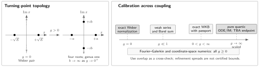
Turning-point and method calibration for $H(g)$. The method bands indicate domains of convenience, not theorem boundaries. In particular, numerical methods work throughout $g\geq0$, while the closed TBA of Chapter 13 belongs to the scaled pure-quartic endpoint rather than generic finite $g$.

The four locations alone do not determine an exact-WKB quantization condition. One must still fix cycles, Stokes chamber, summation direction, and the two real-line decay conditions. The real action below is therefore a controlled leading approximation, not the complete genus-one passport.

Leading WKB improves up the spectrum

The positive turning point satisfies $E=a^2+ga^4$. Define the allowed-region action

$$A(E,g)= \int_{-a}^{a} \sqrt{E-x^2-gx^4}\,\dd x.$$

The substitution $x=a\sin\theta$ removes the endpoint square root:

$$\begin{aligned} A(E,g) =2a^2\int_0^{\pi/2} &\cos^2\theta \\ &\times \sqrt{1+ga^2(1+\sin^2\theta)}\,\dd\theta. \end{aligned}$$

Leading Bohr–Sommerfeld quantization imposes

$$A(E,g)=\pi\left(n+\frac12\right).$$

At $g=0$, $A=\pi E/2$, so this gives $E_n=2n+1$ exactly. The exactness is special to the quadratic potential; the half-integer shift still encodes turning-point connection data. At positive $g$, the comparison is

$g$	direct $E_0$	WKB $E_0$	direct $E_3$	WKB $E_3$
$0$	$1.0000000000$	$1.0000000000$	$7.0000000000$	$7.0000000000$
$0.01$	$1.0073736721$	$1.0037237973$	$7.1785731807$	$7.1754222907$
$0.1$	$1.0652855095$	$1.0351556615$	$8.3526778258$	$8.3383786692$
$1$	$1.3923516415$	$1.2507687598$	$13.1568038981$	$13.1231403072$
$10$	$2.4491740721$	$2.0611395630$	$25.8062762151$	$25.7343596266$

The ground-state error grows with coupling, but the fourth level is already within $0.3\%$ at $g=10$. This is precisely the distinction between a large-level semiclassical statement and a uniformly accurate low-level formula.

For fixed $g>0$ and $n\to\infty$, the quartic term controls the action. Put

$$I_4 =\int_0^1\sqrt{1-t^4}\,\dd t =\frac14B\!\left(\frac14,\frac32\right) =0.874019184764\ldots.$$

Then polynomial spectral asymptotics give

$$E_n(g) \sim g^{1/3} \left[ \frac{\pi(n+1/2)}{2I_4} \right]^{4/3}.$$

This limit does not commute with $g\to0$. At fixed $n$, weak coupling gives $E_n\to2n+1$; at any fixed $g>0$, sufficiently high levels grow as $n^{4/3}$. The crossover estimate $gn\sim1$ agrees with the perturbative moment estimate above.

Expert check: the determinant order jumps at the endpoint

For $g>0$, $E_n\asymp n^{4/3}$, so $\sum_n E_n^{-s}$ converges for $s>3/4$. The normalized genus-zero Fredholm determinant has order $3/4$. At $g=0$, $E_n\asymp n$; the order is one, the direct product requires genus one, and a zero-free exponential participates in the gamma-function normalization.

Thus every fixed eigenvalue converges as $g\to0^+$, while the most economical global product representation changes discontinuously. The genus-zero products themselves need not converge to the harmonic zeta determinant: their logarithmic derivatives at zero contain $-\sum_nE_n(g)^{-1}$, which diverges as $g\downarrow0$. The high-energy tail must instead be absorbed into a $g$-dependent zero-free renormalization.

Strong coupling lands on the pure-quartic endpoint

For $g>0$, set $x=g^{-1/6}y$ and $\eta=g^{-2/3}$. The identity

$$H(g) =g^{1/3} \left[ -\frac{\dd^2}{\dd y^2}+y^4+\eta y^2 \right]$$

turns strong coupling into ordinary fixed-level perturbation theory around the pure-quartic operator $H_4=-\partial_y^2+y^4$. If $H_4\phi_{n,4}=e_n^{(4)}\phi_{n,4}$, then

$$E_n(g) = g^{1/3}e_n^{(4)} +g^{-1/3}\mu_n +O(g^{-1}), \qquad \mu_n=\langle\phi_{n,4},y^2\phi_{n,4}\rangle.$$

Chapter 13 supplies $e_0^{(4)}=1.060362090484\ldots$; the independent calibration below gives $\mu_0=0.362022648789\ldots$. For $g=100$, the two-term result $4.999760254091$ differs from the direct $4.999417545137$ by $3.43\times10^{-4}$.

The scaling imports a spectral endpoint, not an unchanged integral equation. At finite $g$, the scaled potential $y^4+\eta y^2$ has a nontrivial rotated-coupling orbit and different period data. The two-function pure-quartic TBA cannot be reused merely by inserting $\eta$ into its drive term.

Two numerical representations set the standard

The companion program anharmonic-oscillator-calibration.py uses NumPy only:

python3 public/code/advanced-ode/anharmonic-oscillator-calibration.py
python3 public/code/advanced-ode/anharmonic-oscillator-calibration.py --high

The first representation is a half-line Fourier–Galerkin box $0\leq x\leq L$. Both bases vanish at the artificial wall $x=L$; at $x=0$ the cosine basis is Neumann and the sine basis is Dirichlet, encoding even and odd parity:

$$\begin{aligned} \phi_j^{\mathrm N}(x) &=\sqrt{\frac2L} \cos\frac{(j+1/2)\pi x}{L}, \\ \phi_j^{\mathrm D}(x) &=\sqrt{\frac2L} \sin\frac{(j+1)\pi x}{L}. \end{aligned}$$

The kinetic matrix is diagonal. With $c_p(m)=L^{-1}\int_0^Lx^p\cos(m\pi x/L)\,\dd x$, the potential matrices are exact:

$$\begin{aligned} (V_p^{\mathrm N})_{jk} &=c_p(j-k)+c_p(j+k+1), \\ (V_p^{\mathrm D})_{jk} &=c_p(j-k)-c_p(j+k+2). \end{aligned}$$

Here

$$\begin{gathered} c_2(0)=\frac{L^2}{3}, \qquad c_4(0)=\frac{L^4}{5}, \\ c_2(m)= \frac{2L^2(-1)^m}{(m\pi)^2}, \qquad m\ne0, \\ c_4(m)= L^4(-1)^m \left[ \frac4{(m\pi)^2}-\frac{24}{(m\pi)^4} \right], \qquad m\ne0. \end{gathered}$$

The independent representation uses a full-line coordinate grid with Dirichlet walls. Its tridiagonal entries are

$$\begin{aligned} (H_h)_{ii} &=\frac2{h^2}+x_i^2+gx_i^4, \\ (H_h)_{i,i\pm1} &=-\frac1{h^2}. \end{aligned}$$

Sturm counts and bisection find only the requested low eigenvalues. Three nested meshes allow the $h^2$ and $h^4$ terms to be canceled without a dense diagonalization.

With $L=8(1+g)^{-1/6}$ and $60$ functions per parity block, the program returns

$g$	$E_0$	$E_1$	$E_2$	$E_3$
$0$	$1.0000000000$	$3.0000000000$	$5.0000000000$	$7.0000000000$
$0.01$	$1.0073736721$	$3.0365253045$	$5.0939391327$	$7.1785731807$
$0.1$	$1.0652855095$	$3.3068720132$	$5.7479592688$	$8.3526778258$
$1$	$1.3923516415$	$4.6488127042$	$8.6550499578$	$13.1568038981$
$10$	$2.4491740721$	$8.5990034548$	$16.6359214924$	$25.8062762151$
$100$	$4.9994175451$	$17.8301927160$	$34.8739842620$	$54.3852915716$

Across this grid and these four levels, the largest changes are

Audit	Maximum observed change
$60$ versus $48$ Fourier functions	$6.9\times10^{-12}$
box scale $8$ versus $7$	$3.9\times10^{-12}$
final versus previous coordinate extrapolation	$7.7\times10^{-9}$
final coordinate versus Fourier–Galerkin value	$5.8\times10^{-11}$
Fourier virial residual	$8.0\times10^{-12}$

The raw coordinate correction is much larger than the final inter-method discrepancy; reporting only the latter would hide the discretization path. Conversely, a refinement shift is not automatically an upper error bound. The values are reproducible to about nine or ten digits, but they are not interval-certified. The evidence hierarchy and escalation route are given on the verified-numerics page.

Choose the method from the question

Regime or goal	Efficient method	What must not be inferred
$g=0$	Exact Weber/Hermite solution	A generic four-turning-point formula is unnecessary
Fixed $n$, $0<g\ll1$	Optimal truncation or Borel-resummed perturbation theory	The raw series does not converge
Any real $g\geq0$	Independently refined spectral and coordinate numerics	Decimal agreement is not interval certification
Fixed $g>0$, large $n$	WKB and polynomial spectral asymptotics	Leading WKB need not be accurate for low levels
Exact finite-$g$ connection data	Exact WKB with cycle, chamber, summation, and boundary passports	The real action alone is incomplete
Determinant questions	Parity-resolved spectral determinants with fixed normalization	Zeros do not fix zero-free factors
Scaled $g\to\infty$	Pure-quartic exact WKB, ODE/IM, and TBA	The pure-quartic TBA is not a finite-$g$ formula

Common pitfalls

Mixing oscillator conventions. The Hamiltonians $-\partial_x^2+x^2+gx^4$ and $-\tfrac12\partial_x^2+\tfrac12x^2+\lambda x^4$ are related by an energy and coupling rescaling. Copying Bender–Wu coefficients or quartic levels without this ledger gives internally plausible but wrong numbers.

Calling asymptotic series inaccurate Taylor series. A Taylor series has a convergence question; this Rayleigh–Schrödinger series has zero radius and an asymptotic meaning. Borel summability is the separate theorem that recovers the stable eigenvalue.

Treating four roots as an exact quantization condition. Turning points define the spectral curve, but exact WKB also needs cycles, Stokes chamber, summation direction, and boundary data. Leading real-action quantization does not contain the full complex-cycle information.

Transporting endpoint structures to finite coupling. The strong scaling lands on the pure quartic only as $\eta=g^{-2/3}\to0$. Its determinant and TBA identities require a fresh derivation once the $\eta y^2$ term is present.

Exercises

1. Restore physical units

Starting from $H_{\mathrm{phys}}$, derive the dimensionless coupling and convert a computed dimensionless level back to physical energy.

Solution

Put $q=\ell x$ with $\ell^2=\hbar/(m\omega)$. Both the kinetic and quadratic terms become $(\hbar\omega/2)(-\partial_x^2+x^2)$. The quartic coefficient inside the same bracket is

$$g= \frac{\lambda_{\mathrm{phys}}\ell^4} {\hbar\omega/2} =\frac{2\lambda_{\mathrm{phys}}\hbar}{m^2\omega^3}.$$

Therefore $E_n^{\mathrm{phys}}=(\hbar\omega/2)E_n(g)$.

2. Derive the five diagonals

Use the harmonic ladder operators to derive the three displayed upper-triangular entries of $H(g)$ and prove parity decoupling.

Solution

First apply

$$x^2|n\rangle =\frac12 \left[ \sqrt{n(n-1)}|n-2\rangle +(2n+1)|n\rangle +\sqrt{(n+1)(n+2)}|n+2\rangle \right].$$

Applying $x^2$ once more gives

$$\begin{aligned} \langle n|x^4|n\rangle &=\frac34(2n^2+2n+1), \\ \langle n|x^4|n+2\rangle &=\frac12(2n+3)\sqrt{(n+1)(n+2)}, \\ \langle n|x^4|n+4\rangle &=\frac14\sqrt{(n+1)(n+2)(n+3)(n+4)}. \end{aligned}$$

All shifts are even, so even and odd $n$ form invariant blocks.

3. Recover the second weak coefficient

Evaluate the second-order Rayleigh–Schrödinger sum for level $n$.

Solution

Only $m=n\pm2,n\pm4$ contribute, and $E_n^{(0)}-E_m^{(0)}=2(n-m)$. Thus

$$E_n^{(2)} = \sum_{m\ne n} \frac{|\langle m|x^4|n\rangle|^2} {E_n^{(0)}-E_m^{(0)}}.$$

Insert the matrix elements from Exercise 2, omit states with negative indices, and simplify. The result, whose polynomial also gives the correct boundary cases $n=0,1$, is

$$E_n^{(2)} =-\frac{34n^3+51n^2+59n+21}{16}.$$

For $n=0$ this is $-21/16$.

4. Reconstruct the ground-state recurrence

Write $\psi=\ee^{-x^2/2}\sum_{k\geq0}g^kf_k(x)$ with $f_0=1$ and $f_k(0)=0$ for $k>0$. Derive a coefficient recurrence suitable for exact rational arithmetic.

Solution

After removing the Gaussian, put $L=-\partial_x^2+2x\partial_x$ and $E=1+\sum_{k\geq1}e_kg^k$. At order $k$,

$$Lf_k = \sum_{j=1}^{k}e_jf_{k-j}-x^4f_{k-1}.$$

Write $f_k=\sum_{m=1}^{2k}a_{k,m}x^{2m}$. The constant term gives $e_k=-2a_{k,1}$. For $m\geq1$, define

$$r_{k,m} = \sum_{j=1}^{k-1}e_j a_{k-j,m} -a_{k-1,m-2},$$

with absent coefficients set to zero. Descending from $m=2k$,

$$a_{k,m} = \frac{ r_{k,m}+2(m+1)(2m+1)a_{k,m+1} }{4m}.$$

This produces $e_1=3/4$, $e_2=-21/16$, and the later coefficients printed by the companion program.

5. Follow the roots through weak coupling

Derive $\pm a,\pm\ii b$, find their $g\to0^+$ behavior, and determine the genus of the compactified curve.

Solution

Solving $gz^2+z-E=0$ for $z=x^2$ gives $z=a^2>0$ and $z=-b^2<0$, with the formulas in the text. Rationalizing the first one shows $a^2=2E/(1+\sqrt{1+4gE})\to E$. The second behaves as $b^2=g^{-1}+E+O(g)$, so $b\sim g^{-1/2}$.

A smooth double cover branched at four distinct finite points has genus one. When $g=0$, two branch points escape to infinity and the degree-two curve has genus zero.

6. Expose the noncommuting limits

Derive the leading high-level formula and compare the orders of the spectral determinants at $g=0$ and $g>0$.

Solution

In the quartic-dominated regime, put $x=(E/g)^{1/4}t$. The allowed action becomes

$$A(E,g) \sim2E^{3/4}g^{-1/4}I_4.$$

Equating it to $\pi(n+1/2)$ gives the formula in the text. Hence $E_n\asymp n^{4/3}$ for every fixed $g>0$, whereas $E_n(0)\asymp n$. The corresponding convergence exponents are $3/4$ and $1$, giving determinant orders $3/4$ and $1$ and minimal product genera zero and one. Fixed-$n$ weak coupling therefore cannot be uniform through the high-level limit.

7. Audit the numerical spectrum

Run both default and high modes of the companion program. Explain why the five reported diagnostics test different failure modes.

Solution

The basis-size shift detects Fourier truncation; the box shift detects the artificial wall; the coordinate extrapolation shift measures unresolved mesh error; the inter-method discrepancy compares two representations; and the virial residual probes the eigenvectors, not just their eigenvalues. The exact $g=0$ row catches energy and parity conventions, while monotonicity in $g$ catches ordering or assembly errors.

Agreement of these checks supports the printed digits but does not turn the calculation into interval arithmetic. Certification would require outward rounding and residual or enclosure theorems of the kind described in Chapter 4.

8. Gate the strong-coupling import

Derive the first correction about the pure quartic and state which Chapter 13 structures may be imported at finite $g$.

Solution

The scaling $x=g^{-1/6}y$ gives $E_n(g)=g^{1/3}\mathcal E_n(\eta)$ with $\eta=g^{-2/3}$. Ordinary first-order perturbation theory for $H_4+\eta y^2$ yields

$$\mathcal E_n(\eta) =e_n^{(4)}+\eta\langle\phi_{n,4},y^2\phi_{n,4}\rangle+O(\eta^2).$$

Thus the pure-quartic energies and matrix elements are legitimate endpoint inputs. Its two-function TBA, symmetry folding, exact quantization curve, and determinant functional relation are model-specific identities; none follows for finite $\eta$ without rederiving the rotated sectors, periods, and integral equations.

References

• C. M. Bender and T. T. Wu, “Anharmonic Oscillator”, Physical Review 184 (1969), 1231–1260. Equations (2.3)–(2.12) develop the coefficient recurrence and high-order data; the precise large-order prefactor there is numerical evidence rather than a rigorous bound.
• B. Simon, “Coupling Constant Analyticity for the Anharmonic Oscillator”, Annals of Physics 58 (1970), 76–136. Establishes the operator-theoretic realization, cut-plane analyticity, nonanalyticity at zero, and genuine Rayleigh–Schrödinger asymptotics.
• S. Graffi, V. Grecchi, and B. Simon, “Borel Summability: Application to the Anharmonic Oscillator”, Physics Letters B 32 (1970), 631–634. Proves Borel summability for the quartic and Borel–Leroy summability for higher even monomials.
• C. M. Bender and T. T. Wu, “Anharmonic Oscillator. II. A Study of Perturbation Theory in Large Order”, Physical Review D 7 (1973), 1620–1636. Gives the dispersion framework and detailed large-order WKB prediction; the paper explicitly does not claim growth bounds for its full asymptotic formula.
• A. Voros, “The Return of the Quartic Oscillator: The Complex WKB Method”, Annales de l’Institut Henri Poincaré A 39 (1983), 211–338. Develops the global complex-WKB and determinant structures behind exact anharmonic quantization.
• P. Dorey and R. Tateo, “Anharmonic Oscillators, the Thermodynamic Bethe Ansatz, and Nonlinear Integral Equations”, Journal of Physics A 32 (1999), L419–L425, arXiv:hep-th/9812211. Supplies the homogeneous-oscillator asymptotics, quartic benchmark, and ODE/IM–TBA identification used at the strong endpoint.
• K. C. Shin, “Schrödinger Type Eigenvalue Problems with Polynomial Potentials: Asymptotics of Eigenvalues”, Theorem 1.2. Gives a rigorous polynomial-eigenvalue asymptotic whose self-adjoint specialization reproduces the leading WKB coefficient.

The confining real-line problem selects one decaying line at each endpoint and produces isolated simple levels. A periodic potential replaces those endpoint lines by one-period monodromy and a Bloch multiplier. The next page therefore changes the characteristic scalar from an $L^2$ boundary determinant to the Hill discriminant $\Delta(E)=\operatorname{tr}M(E)$; periodic and antiperiodic band edges occur at $\Delta(E)=\pm2$.