Spectral Theory for Boundary and Resonance Problems

A differential equation has local solutions and connection data, but it does not have a spectrum by itself. Spectral statements begin only after one chooses a function space, a closed domain, boundary or radiation conditions, the way the spectral parameter enters, and—when continuation is involved—a spectral sheet. Changing any one of these can change the answer without changing the printed ODE.

This interlude supplies the operator layer needed by the rest of the book. It starts with self-adjoint Sturm–Liouville realizations, passes through singular endpoints and analytic operator pencils, and ends with nonselfadjoint resonances and black-hole quasinormal boundary conditions. The next page will turn selected boundary solutions into analytic functions; here the task is to say what those functions are meant to detect.

A spectral problem is a stack of choices

A useful ledger is

$$\begin{aligned} \mathfrak P =\bigl( &\text{differential expression}, \text{ function space}, \text{ closed domain},\\ &\text{parameter dependence}, \text{ boundary data}, \text{ spectral sheet} \bigr). \end{aligned}$$

Here “closed” refers to the graph of the realized operator. Its domain need not be a closed subspace of the ambient Hilbert space.

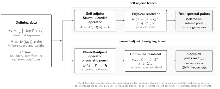
The spectral data stack. Self-adjoint boundary conditions lead to the usual resolvent and real spectral theory; outgoing or ingoing conditions produce a nonselfadjoint pencil whose continued resolvent can have resonance or quasinormal-mode poles.

Several words that are often treated as synonyms occupy different levels:

Object	Minimal meaning	Extra hypotheses often needed
Differential expression	A local rule such as $-y''+Vy$	None; it is not yet an operator
Closed operator	An expression with a domain whose graph is closed	Density is needed for an adjoint
Eigenvalue	A nonzero domain vector solves $(L-\lambda)y=0$	Discreteness needs compactness or another theorem
Pencil characteristic value	$T(\lambda)$ is not invertible	Analytic multiplicity needs a Fredholm family
Resonance	A pole on a declared nonphysical meromorphic continuation	The continuation space and sheet must be stated
Quasinormal frequency	A resonance or equivalent mode satisfying physical asymptotics	The pole–mode equivalence and time convention must be proved

The regular Sturm–Liouville operator

On a finite interval $(a,b)$, consider the real expression

$$\tau y = \frac1{w(x)} \left[ -\bigl(p(x)y'(x)\bigr)' +q(x)y(x) \right], \qquad p>0,\quad w>0.$$

For the present regular discussion, take finite endpoints and coefficients regular enough that endpoint values exist. The natural Hilbert space is

$$\mathcal H=L^2\bigl((a,b),w(x)\,\dd x\bigr),$$

with

$$\langle f,g\rangle = \int_a^b f(x)\overline{g(x)}w(x)\,\dd x.$$

The maximal domain consists, schematically, of functions for which $y$ and $py'$ are absolutely continuous and $\tau y\in\mathcal H$. The maximal realization is closed but generally not symmetric. Self-adjoint realizations are obtained by restricting its domain with maximal isotropic boundary conditions.

The boundary form decides symmetry

Integration by parts gives Green’s or Lagrange’s identity

$$\begin{aligned} \langle \tau f,g\rangle -\langle f,\tau g\rangle &= \left[ p\left( f\overline{g'} -f'\overline g \right) \right]_{a}^{b}. \end{aligned}$$

Write the endpoint concomitant as

$$[f,g](x) = p(x) \left( f(x)\overline{g'(x)} -f'(x)\overline{g(x)} \right).$$

A symmetric domain makes $[f,g](b)-[f,g](a)$ vanish for every pair $f,g$ in the domain. A self-adjoint domain must additionally equal the domain of its adjoint. Reality of $p,q,w$ is therefore necessary for this elementary self-adjoint setup, but it is not sufficient.

For a compact matrix test, set

$$Y_f(x) = \begin{pmatrix} f(x)\\ (pf')(x) \end{pmatrix}, \qquad J= \begin{pmatrix} 0&-1\\ 1&0 \end{pmatrix}.$$

Then $[f,g](x)=Y_g(x)^*JY_f(x)$. A regular two-point condition

$$A\,Y_f(a)+B\,Y_f(b)=0$$

is self-adjoint precisely when

$$\operatorname{rank}(A\ B)=2, \qquad AJA^*=BJB^*.$$

Every separated regular self-adjoint condition can be written

$$\cos\alpha\,y(a) +\sin\alpha\,(py')(a)=0,$$

and

$$\cos\beta\,y(b) +\sin\beta\,(py')(b)=0,$$

for real $\alpha,\beta$, with angles understood modulo $\pi$. Dirichlet, Neumann, and real Robin conditions are special cases.

Self-adjoint conditions need not be separated. Set

$$\mathbf v_y(x) = \begin{pmatrix} y(x)\\ p(x)y'(x) \end{pmatrix}.$$

A standard coupled family is

$$\mathbf v_y(b) = \ee^{\ii\vartheta} R\,\mathbf v_y(a), \qquad R\in SL(2,\mathbb R), \quad \vartheta\in[0,\pi).$$

The determinant-one condition preserves the endpoint symplectic form. Because $(\vartheta,R)\sim(\vartheta+\pi,-R)$, the half-open phase interval is sufficient. Periodic and antiperiodic domains occur at $(\vartheta,R)=(0,I)$ and $(0,-I)$.

One expression, three spectra

Take $\tau=-\dd^2/\dd x^2$ in $L^2(0,L)$. The differential expression is unchanged in the following three problems:

Domain condition	Eigenfunctions	Eigenvalues
$y(0)=y(L)=0$	$\sqrt{2/L}\sin(n\pi x/L)$, $n\ge1$	$(n\pi/L)^2$
$y'(0)=y'(L)=0$	$L^{-1/2}$ for $n=0$; $\sqrt{2/L}\cos(n\pi x/L)$ for $n\ge1$	$(n\pi/L)^2$, $n\ge0$
$y(0)=y(L)$ and $y'(0)=y'(L)$	$L^{-1/2}\ee^{2\pi\ii n x/L}$, $n\in\mathbb Z$	$(2\pi n/L)^2$

The periodic nonzero eigenvalues have multiplicity two because $n$ and $-n$ give independent eigenfunctions. This elementary table is the quickest counterexample to the phrase “the spectrum of the equation.”

Singular endpoints choose how much boundary data remain

An endpoint is singular if the regular endpoint assumptions fail—for example, the interval is unbounded or a coefficient degenerates. Endpoint values may then be meaningless, so the maximal-domain boundary form must be defined by limits rather than by substituting into a Robin formula.

For one—and hence every—nonreal $\lambda$, an endpoint is limit-circle if every local solution of

$$\tau y=\lambda y$$

is square-integrable there. Otherwise it is limit-point. For a scalar second-order real Sturm–Liouville problem:

• a limit-point endpoint requires no separated boundary condition for a self-adjoint realization;
• a limit-circle endpoint requires one boundary condition; and
• a regular endpoint is limit-circle.

At a limit-point endpoint, the limiting bracket vanishes automatically for maximal-domain functions. Each limit-circle endpoint contributes one to both deficiency indices. If both endpoints are limit-point, the minimal operator is essentially self-adjoint. None of these statements determines whether the resulting spectrum is discrete or continuous.

The slogan “choose the regular solution” is too vague when both solutions are square-integrable. The required condition is a statement about the operator domain and the limiting boundary form.

The inverse-square threshold

Consider

$$\tau_g = -\frac{\dd^2}{\dd x^2} +\frac{g}{x^2}$$

in $L^2(0,\infty)$. For $g\ge-1/4$, set

$$\nu=\sqrt{g+\frac14}.$$

Near zero the two leading behaviors are

$$x^{1/2+\nu}, \qquad x^{1/2-\nu},$$

with the second replaced by $x^{1/2}\log x$ at $\nu=0$. Both lie in $L^2(0,\varepsilon)$ exactly when $\nu<1$. Hence

$$\begin{array}{c|c} -\dfrac14\le g<\dfrac34 &\text{limit-circle at }0,\\ g\ge\dfrac34 &\text{limit-point at }0. \end{array}$$

Infinity is limit-point for this model. Thus the operator initially defined on $C_c^\infty(0,\infty)$ is essentially self-adjoint for $g\ge3/4$; below that threshold, one boundary condition at zero selects an extension. For $g<-1/4$, both oscillatory powers $x^{1/2\pm\ii\sqrt{-g-1/4}}$ are locally square-integrable, but semiboundedness fails and the extension problem needs additional care.

Spectrum begins with a closed operator

For a closed, densely defined operator $L:\mathcal D(L)\subset\mathcal H\to\mathcal H$, the resolvent set is

$$\begin{aligned} \rho(L) = \bigl\{ \lambda\in\mathbb C: &\,L-\lambda \text{ is bijective,}\\ &\,(L-\lambda)^{-1} \in\mathcal B(\mathcal H) \bigr\}. \end{aligned}$$

The spectrum is $\sigma(L)=\mathbb C\setminus\rho(L)$. An eigenvalue is a spectral point with a nonzero vector $y\in\mathcal D(L)$ satisfying

$$(L-\lambda)y=0.$$

Self-adjointness forces the spectrum to be real and gives the resolvent estimate

$$\left\| (L-z)^{-1} \right\| \le \frac1{|\operatorname{Im}z|}, \qquad \operatorname{Im}z\ne0.$$

It does not force the spectrum to consist only of eigenvalues. Discreteness follows from an additional property such as compact resolvent. Regular Sturm–Liouville realizations on a finite interval have compact resolvent, but half-line and whole-line operators commonly have continuous spectrum.

For nonselfadjoint operators, eigenvectors need not be orthogonal or complete, algebraic and geometric multiplicities can differ, and the resolvent can be large far from the spectrum. The $\varepsilon$-pseudospectrum,

$$\sigma_\varepsilon(L) = \sigma(L) \cup \left\{ z\in\rho(L): \left\|(L-z)^{-1}\right\|>\varepsilon^{-1} \right\},$$

records this instability. A numerically stable-looking list of complex roots is not by itself an operator-theoretic spectral theorem.

Analytic pencils allow nonlinear spectral parameters

Many separated equations are not of the form $L-\lambda$. Rotation, dissipation, gauge constraints, frequency-dependent boundary conditions, and elimination of coupled fields can produce an analytic operator pencil

$$T(\lambda):\mathcal D\longrightarrow\mathcal H.$$

The domain $\mathcal D$ must be fixed. For an unbounded problem, equip it with a graph norm so that $T(\lambda)$ is a bounded map from $\mathcal D$ to $\mathcal H$. If the differential expression and boundary conditions both depend on $\lambda$, one useful fixed-domain formulation is

$$\mathcal T(\lambda)y = \bigl( T(\lambda)y, B(\lambda)y \bigr): \mathcal D_{\max} \longrightarrow \mathcal H\oplus\mathbb C^r.$$

Hiding a varying boundary condition inside a varying domain can destroy the holomorphic-family hypothesis.

The analytic Fredholm alternative

Let $\Omega\subset\mathbb C$ be a connected open set. Suppose $T(\lambda):X\to Y$ is a norm-holomorphic family of Fredholm operators of index zero between fixed Banach spaces. Then exactly one of the following occurs:

1. $T(\lambda)$ is noninvertible for every $\lambda\in\Omega$; or
2. if it is invertible at one point, its inverse is finitely meromorphic on $\Omega$, and the noninvertible set is discrete.

The principal parts of the inverse have finite rank. The “invertible somewhere” test is indispensable: Fredholmness alone does not prevent every parameter value from being characteristic.

Let $\lambda_0$ be an isolated characteristic value and let $\Gamma_0$ be a small positively oriented circle enclosing no other one. Under the standard finite-type hypotheses, its algebraic multiplicity is

$$m(\lambda_0;T) = \operatorname{tr} \left[ \frac{1}{2\pi\ii} \oint_{\Gamma_0} T'(\lambda) T(\lambda)^{-1}\,\dd\lambda \right].$$

The trace is taken after integration; the pointwise integrand need not be trace class. For the linear pencil $T(\lambda)=L-\lambda$,

$$T'(\lambda)T(\lambda)^{-1} =(\lambda-L)^{-1},$$

so the contour integral is the Riesz projection. For a nonlinear pencil, a chain $(u_0,\ldots,u_{m-1})$ satisfies

$$\sum_{j=0}^{k} \frac1{j!} T^{(j)}(\lambda_0)u_{k-j} =0, \qquad k=0,\ldots,m-1.$$

The $k=0$ equation is $T(\lambda_0)u_0=0$; the next is

$$T(\lambda_0)u_1 +T'(\lambda_0)u_0 =0.$$

Thus $\dim\ker T(\lambda_0)$ is only the geometric multiplicity. Algebraic multiplicity, inverse pole order, and residue rank need not agree.

The finite-dimensional pencil

$$A(\lambda) = \begin{pmatrix} \lambda^2&0\\ 0&\lambda \end{pmatrix}$$

makes all three distinctions visible at $\lambda=0$. Its kernel has dimension two, while

$$A'(\lambda)A(\lambda)^{-1} = \begin{pmatrix} 2/\lambda&0\\ 0&1/\lambda \end{pmatrix}$$

gives algebraic multiplicity three. Meanwhile $A^{-1}$ has pole order two and residue $\operatorname{diag}(0,1)$ of rank one.

Resonances are poles on a continued sheet

Let $P$ be a self-adjoint scattering operator. Its physical resolvent is initially defined away from $\sigma(P)$. A resonance theory begins only after a cutoff or weighted resolvent has been continued meromorphically through part of the continuous spectrum, often on a branched cover of the energy plane. A resonance is a pole of that declared continuation.

We will reserve “resonance” for a pole on a nonphysical continuation and call a physical-sheet pole an eigenvalue. Some sources include the latter in the resonance set, so this convention must be checked when comparing statements.

The qualifiers are part of the definition:

• which resolvent or scattering matrix is continued;
• between which weighted, cutoff, or compactly supported spaces;
• which parameter is used, such as energy $z$ or wave number $k$ with $z=k^2$;
• across which threshold or branch cut; and
• how pole multiplicity is counted.

Such a continuation is a theorem for a specified class of operators, not a formal consequence of writing an outgoing exponential. In even spatial dimensions it commonly lives on a logarithmic cover, while thresholds such as $k=0$ need separate treatment.

A one-dimensional outgoing model

Let

$$P=-\frac{\dd^2}{\dd x^2}+V(x)$$

on the line, with $V\in L^\infty_c(\mathbb R;\mathbb R)$. For $\operatorname{Im}k>0$ wherever $k^2\in\rho(P)$, the physical resolvent

$$R_V(k)=(P-k^2)^{-1}$$

acts in particular from compactly supported to locally square-integrable functions. Choose Jost solutions

$$\begin{aligned} f_-(x,k)&\sim\ee^{-\ii kx} && (x\to-\infty),\\ f_+(x,k)&\sim\ee^{+\ii kx} && (x\to+\infty). \end{aligned}$$

With the book’s Wronskian convention, its outgoing Green kernel is

$$G(x,y;k) = -\frac{ f_-(x_<,k)f_+(x_>,k) }{ \Wr[f_-,f_+](k) },$$

where

$$x_<=\min(x,y), \qquad x_>=\max(x,y).$$

The minus sign makes the derivative jump solve $(P-k^2)G=\delta$. The cutoff resolvent continues meromorphically in $k$ for this compactly supported one-dimensional model. Its poles are resonances. Zeros of the continued Jost Wronskian produce those poles unless a numerator cancellation intervenes.

For $\operatorname{Im}k<0$, the outgoing exponentials grow at their respective spatial ends. A resonant state is therefore generally not an $L^2$ eigenfunction. Moreover, $k$ and $-k$ correspond to the same energy $k^2$ but opposite radiation conditions.

A Robin pole crosses the square-root sheets

On the half-line, let

$$\begin{aligned} H_h&=-\frac{\dd^2}{\dd x^2},\\ \mathcal D(H_h) &= \left\{ u\in H^2(0,\infty): u'(0)=h\,u(0) \right\}, \qquad h\in\mathbb R. \end{aligned}$$

This is a self-adjoint operator. For $\operatorname{Im}k>0$ and $k\ne0$, with $k^2\in\rho(H_h)$, its outgoing resolvent kernel is

$$\begin{aligned} G_h(k;x,y) = \frac{\ii}{2k} \biggl[ &\ee^{\ii k|x-y|}\\ &+ \frac{k-\ii h}{k+\ii h} \ee^{\ii k(x+y)} \biggr]. \end{aligned}$$

Direct differentiation gives

$$\partial_xG_h(k;0,y) = h\,G_h(k;0,y).$$

For $h\ne0$, the continued kernel has a nonthreshold pole at $k=-\ii h$. If $h<0$, the pole lies on the physical upper half-plane and $u(x)=\ee^{hx}$ is an $L^2$ eigenfunction with energy $-h^2$. If $h>0$, the same formal energy lies at a lower-half-plane pole; its outgoing state $\ee^{hx}$ grows and is not in $L^2$. It is often called a virtual or antibound state. At $h=0$, the pole reaches the threshold $k=0$. The domain, wave-number sheet, and radiation condition—not the energy $k^2=-h^2$ alone—make the distinction.

This formula explains why a boundary Wronskian can represent a resonance. It does not license that interpretation for an arbitrary ODE: the continued resolvent and the equivalence of its poles with Wronskian zeros still have to be established.

Quasinormal modes are convention-locked resonances

Consider a separated wave equation with time dependence $\ee^{-\ii\omega t}$ and a tortoise coordinate $r_*$. In an asymptotically flat black-hole model, a typical radial equation has the form

$$\frac{\dd^2\psi}{\dd r_*^2} +\bigl(\omega^2-V(r_*)\bigr)\psi =0.$$

For a nonrotating horizon, the usual quasinormal conditions are

$$\begin{aligned} \psi(r_*)&\sim\ee^{-\ii\omega r_*} && (r_*\to-\infty), &&\text{future-horizon ingoing},\\ \psi(r_*)&\sim\ee^{+\ii\omega r_*} && (r_*\to+\infty), &&\text{spatial-infinity outgoing}. \end{aligned}$$

The signs follow from the null coordinates $v=t+r_*$ and $u=t-r_*$. With the chosen $\ee^{-\ii\omega t}$ convention, temporal decay means $\operatorname{Im}\omega<0$. Reversing the time Fourier convention reverses the printed radial signs and the decaying half-plane.

These conditions are nonselfadjoint. Decaying quasinormal modes usually grow in $r_*$ at both ends and are not Hilbert-space eigenfunctions of the physical self-adjoint wave operator. “Ingoing at the horizon” is more invariantly future-horizon regularity. In rotating or charged problems, the horizon phase contains a shifted frequency such as $\omega-m\Omega_H-q\Phi_H$, not simply $\omega$.

The outer condition depends on the spacetime. Asymptotically de Sitter problems use a cosmological-horizon radiation condition; asymptotically AdS problems instead require a declared admissible boundary condition, such as Dirichlet, Robin, normalizability, or a holographically selected quantization. “Outgoing at infinity” is not a universal QNM prescription.

When a meromorphic continuation of the stationary resolvent or retarded Green function has been constructed, its poles define quasinormal frequencies and justify the mode condition. In other frameworks QNMs are eigenvalues of a time-translation generator on a carefully chosen space. Equivalence between these definitions is a theorem in particular settings.

Exceptional frequencies, thresholds, gauge modes, and branch cuts can spoil a naive one-to-one identification. Higher-order poles or Jordan chains produce polynomial factors multiplying $\ee^{-\ii\omega t}$. A discrete pole set does not imply completeness, and late-time tails from branch cuts are not captured by a pure QNM sum.

A spectral audit ledger

Before calling a complex number an eigenvalue, resonance, or quasinormal frequency, record:

Datum	Question to answer
Expression	Which scalar or matrix differential expression is used?
Function space	What measure, weight, regularity, or weighted space is intended?
Domain	Which endpoint, interface, gauge, and regularity conditions make the operator closed?
Parameter	Does the problem use $\lambda$, $k$, $\lambda=k^2$, or a nonlinear pencil?
Analytic family	Is the domain fixed, the family Fredholm, and one value invertible?
Continuation	Which resolvent continues, between which spaces, and onto which sheet?
Boundary modes	Which normalized local solutions are selected at each end?
Multiplicity	Is it a kernel dimension, Riesz rank, pole order, or contour index?
Verification	Which independent operator, Wronskian, or numerical check is available?

The connection matrices from the preceding pages become spectral only after this ledger selects an entry and supplies its analytic meaning.

Common pitfalls

Taking the spectrum of a differential expression. The Dirichlet, Neumann, and periodic interval examples have the same expression and different spectra. Always name the space and closed domain.

Imposing a boundary condition at a limit-point endpoint. A separated self-adjoint realization needs no condition there. Adding one can overdetermine the domain or define a different, nonselfadjoint problem.

Calling real coefficients self-adjoint. Symmetry requires the boundary form to vanish, and self-adjointness requires the adjoint domain to coincide. Endpoint classification and domain maximality are essential.

Applying analytic Fredholm theory to a moving domain. Reformulate frequency-dependent boundary data as an augmented map on a fixed maximal domain. Then verify Fredholmness, index zero, and invertibility somewhere.

Calling every outgoing solution a resonance. A resonance is a pole of a specified meromorphic continuation. The outgoing mode is equivalent only after an operator theorem connects the two.

Forgetting Fourier and sheet conventions. The signs of ingoing and outgoing exponentials and the decaying half-plane depend on $\ee^{-\ii\omega t}$ versus $\ee^{+\ii\omega t}$. Energy and wave-number planes also have different branch structures.

Exercises

1. Make separated boundary conditions isotropic. Let $f$ and $g$ satisfy the same separated real conditions with angles $\alpha$ and $\beta$. Prove directly from the endpoint vectors that the Lagrange boundary form vanishes. Why does this give a self-adjoint, rather than merely symmetric, regular realization?

Solution

At the left endpoint, the condition says that both endpoint vectors lie in the complex line spanned by

$$q_\alpha = \begin{pmatrix} -\sin\alpha\\ \cos\alpha \end{pmatrix}.$$

Thus $Y_f(a)=c_fq_\alpha$ and $Y_g(a)=c_gq_\alpha$. Since $q_\alpha^{T}Jq_\alpha=0$,

$$[f,g](a) = \overline{c_g}c_f q_\alpha^{T}Jq_\alpha =0.$$

The same argument with $q_\beta$ gives $[f,g](b)=0$, so Green’s identity proves symmetry. The four-dimensional regular boundary-data space carries the nondegenerate symplectic form $[f,g](b)-[f,g](a)$. The two independent endpoint conditions define a maximal isotropic subspace. Maximality is exactly what makes the adjoint domain no larger, so the realization is self-adjoint.

2. Reconstruct the three interval spectra. Starting from $-y''=\lambda y$ on $(0,L)$, derive the Dirichlet, Neumann, and periodic spectra in the table above, including the zero modes and multiplicities.

Solution

Integration by parts under any of the three boundary conditions gives

$$\int_0^L |y'|^2\,\dd x = \lambda \int_0^L |y|^2\,\dd x,$$

so an eigenvalue is nonnegative. At $\lambda=0$, the affine solutions show that Dirichlet has no nonzero eigenfunction, while Neumann and periodic conditions retain only the constants.

For $\lambda=k^2>0$,

$$y(x)=A\cos(kx)+B\sin(kx).$$

Dirichlet conditions give $A=0$ and $\sin(kL)=0$, hence $k=n\pi/L$ with $n\ge1$. Neumann conditions give $B=0$ and the same positive wave numbers. For periodic data, propagation through one period must fix the initial vector. The propagation matrix is

$$M(k) = \begin{pmatrix} \cos(kL)&\sin(kL)/k\\ -k\sin(kL)&\cos(kL) \end{pmatrix},$$

and

$$\det\bigl(M(k)-I\bigr) = 2-2\cos(kL).$$

Thus $kL=2\pi n$. The zero eigenspace consists of the constants. Every positive eigenvalue corresponds to $n$ and $-n$, or equivalently to the independent functions $\cos(2\pi nx/L)$ and $\sin(2\pi nx/L)$, so it has multiplicity two.

3. Locate the inverse-square transition. Derive the indicial powers for $\tau_g$ at zero and recover the limit-circle threshold $g=3/4$. Explain what happens at the borderline.

Solution

Substitution of $y=x^\rho$ into the leading zero-energy equation gives

$$-\rho(\rho-1)+g=0,$$

so

$$\rho=\frac12\pm\nu, \qquad \nu=\sqrt{g+\frac14}.$$

A power $x^\rho$ with real $\rho$ lies in $L^2(0,\varepsilon)$ exactly when $2\rho>-1$. The plus solution is square-integrable for every $\nu\ge0$, whereas the minus solution is square-integrable precisely when $\nu<1$. Therefore zero is limit-circle for $-1/4\le g<3/4$ and limit-point for $g\ge3/4$. At $g=3/4$, the second behavior is $x^{-1/2}$ and its squared modulus has the divergent integral $\int_0^\varepsilon x^{-1}\,\dd x$, so the borderline belongs to the limit-point case. At $g=-1/4$, the repeated-root solution $x^{1/2}\log x$ remains square-integrable.

4. Separate four multiplicity notions. For

$$B(\lambda) = \begin{pmatrix} \lambda^3&0\\ 0&2+\lambda \end{pmatrix},$$

compute at $\lambda=0$ the kernel dimension, algebraic multiplicity, pole order of $B^{-1}$, and rank of its residue. Exhibit a longest chain.

Solution

The kernel of $B(0)$ is $\mathbb C e_1$, so the geometric multiplicity is one. On a small circle about zero,

$$B'(\lambda)B(\lambda)^{-1} = \begin{pmatrix} 3/\lambda&0\\ 0&1/(2+\lambda) \end{pmatrix}.$$

The contour trace is therefore $3$, equal to the order of the zero of $\det B(\lambda)=\lambda^3(2+\lambda)$. Hence the algebraic multiplicity is three.

Meanwhile,

$$B(\lambda)^{-1} = \begin{pmatrix} \lambda^{-3}&0\\ 0&(2+\lambda)^{-1} \end{pmatrix}$$

has pole order three but zero residue, whose rank is zero. A chain of length three is $(u_0,u_1,u_2)=(e_1,0,0)$. It cannot be extended: the $k=3$ chain equation contains

$$\frac1{3!}B^{(3)}(0)u_0=e_1,$$

which does not lie in the range of $B(0)$. This example separates geometric multiplicity and residue rank from algebraic multiplicity and inverse pole order. Together with the preceding two-channel example, it prevents the four notions from being used as synonyms.

5. Audit the Robin pole. Verify the boundary condition for $G_h$, locate its continued pole, and classify that pole for $h<0$ and $h>0$. What changes at $h=0$?

Solution

For $y>0$ and $x=0$, differentiation of the two exponentials gives

$$\begin{aligned} \partial_xG_h(k;0,y) &= \frac{1-R_h(k)}2\,\ee^{\ii ky},\\ G_h(k;0,y) &= \frac{\ii\bigl(1+R_h(k)\bigr)}{2k}\, \ee^{\ii ky}, \end{aligned}$$

where

$$R_h(k)=\frac{k-\ii h}{k+\ii h}.$$

The identities

$$1-R_h(k)=\frac{2\ii h}{k+\ii h}, \qquad 1+R_h(k)=\frac{2k}{k+\ii h}$$

give $\partial_xG_h=hG_h$. For $h\ne0$, the continued kernel has its nonthreshold pole at $k=-\ii h$. If $h<0$, then $k$ lies in the upper half-plane and $\ee^{\ii kx}=\ee^{hx}$ is square-integrable: the energy $-h^2$ is an eigenvalue. If $h>0$, the pole lies in the lower half-plane and the same outgoing state grows, so this is a virtual or antibound pole rather than an $L^2$ eigenvalue. For $h=0$, the pole meets the threshold $k=0$; it must be treated as a threshold singularity, not as an ordinary isolated nonzero resonance.

6. Derive the quasinormal signs. With time dependence $\ee^{-\ii\omega t}$, use $u=t-r_*$ and $v=t+r_*$ to recover the radial factors at the future horizon and at spatial infinity. Which half-plane describes temporal decay, and how do the decaying modes behave spatially?

Solution

A wave regular and ingoing at the future horizon depends on the advanced coordinate $v$, so

$$\ee^{-\ii\omega v} = \ee^{-\ii\omega t} \ee^{-\ii\omega r_*}.$$

An outgoing wave at spatial infinity depends on the retarded coordinate $u$, so

$$\ee^{-\ii\omega u} = \ee^{-\ii\omega t} \ee^{+\ii\omega r_*}.$$

Since $|\ee^{-\ii\omega t}|=\ee^{(\operatorname{Im}\omega)t}$, temporal decay requires $\operatorname{Im}\omega<0$. Writing $\operatorname{Im}\omega=-\gamma$ with $\gamma>0$, the horizon factor grows like $\ee^{\gamma|r_*|}$ as $r_*\to-\infty$, and the infinity factor grows like $\ee^{\gamma r_*}$ as $r_*\to+\infty$. This spatial growth is why a decaying quasinormal mode is generally not an $L^2$ eigenfunction.

7. Turn a Wronskian zero into a theorem. A computation finds $\Wr[f_-,f_+](k_0)=0$ for two formally outgoing solutions. List what must still be established before calling $k_0$ a resonance, and state the additional test needed to determine its multiplicity.

Solution

One must specify the physical resolvent, its source and target spaces, the continuation domain, the wave-number or energy variable, the branch cut, and the sheet containing $k_0$. A theorem must construct a meromorphic continuation there and identify its homogeneous nullvectors with the chosen outgoing solutions. One must also exclude cancellation between the Wronskian zero and the Green-kernel numerator, and treat thresholds separately.

To determine multiplicity, embed the boundary problem into a fixed-domain Fredholm family and evaluate its local contour index, or equivalently use a proved resonance-projection formula. The order of the scalar Wronskian zero agrees with operator algebraic multiplicity only under such a comparison theorem; neither the kernel dimension nor the pole order alone is a substitute.

References

• A. Zettl, Sturm–Liouville Theory, Mathematical Surveys and Monographs 121, AMS, 2005, for regular and singular domains, Lagrange brackets, and the limit-point/limit-circle alternative.
• G. Teschl, Mathematical Methods in Quantum Mechanics: With Applications to Schrödinger Operators, second edition, Graduate Studies in Mathematics 157, AMS, 2014, for self-adjoint operators, one-dimensional Schrödinger theory, and scattering.
• Q. Kong, H. Wu, and A. Zettl, “Geometric aspects of Sturm–Liouville problems I. Structures on spaces of boundary conditions”, Proceedings of the Royal Society of Edinburgh: Section A Mathematics 130 (2000), 561–589, for separated and coupled boundary conditions.
• T. Kato, Perturbation Theory for Linear Operators, second edition, Springer, 1995, for closed operators, resolvents, and analytic operator families.
• I. C. Gohberg and E. I. Sigal, “An operator generalization of the logarithmic residue theorem and the theorem of Rouché”, Mathematics of the USSR-Sbornik 13 (1971), 603–625, for analytic Fredholm factorization and contour multiplicity.
• A. S. Markus, Introduction to the Spectral Theory of Polynomial Operator Pencils, Translations of Mathematical Monographs 71, AMS, 1988, for chains and algebraic multiplicity of nonlinear pencils.
• S. Dyatlov and M. Zworski, Mathematical Theory of Scattering Resonances, Graduate Studies in Mathematics 200, AMS, 2019; an author-hosted version is also available.
• M. Zworski, “Mathematical study of scattering resonances”, Bulletin of Mathematical Sciences 7 (2017), 1–85, for an accessible survey of continuation, resonant states, and resonance expansions.
• E. Berti, V. Cardoso, and A. O. Starinets, “Quasinormal modes of black holes and black branes”, Classical and Quantum Gravity 26 (2009), 163001, for physical conventions, methods, and applications.
• E. W. Leaver, “An analytic representation for the quasi-normal modes of Kerr black holes”, Proceedings of the Royal Society A 402 (1985), 285–298, for the radiative boundary-value formulation and continued-fraction method.
• S. Dyatlov, “Quasi-normal modes and exponential energy decay for the Kerr–de Sitter black hole”, Communications in Mathematical Physics 306 (2011), 119–163, for a rigorous pole definition and its relation to black-hole wave decay.
• C. M. Warnick, “On quasinormal modes of asymptotically anti-de Sitter black holes”, Communications in Mathematical Physics 333 (2015), 959–1035, for the generator-eigenvalue framework, admissible AdS boundary conditions, and limitations of mode completeness.