Connection Matrices for the General Heun Equation

The general Heun connection problem is not solved by a table of gamma functions alone. The gamma functions give a finite degenerate-fusion operation, but a unit-leading ODE matrix also contains endpoint powers, derivatives of the classical block, an accessory-to-Floquet inversion, and branch data. All of these factors are visible already in the connection from $z=0$ to $z=t$.

This page fixes one concrete convention and carries the assembly to a complete $2\times2$ matrix. The determinant is then computed a second way from Wronskians. That independent check detects a missing power of $t$ or a wrong gamma factor immediately. It cannot detect a transpose; direction and row–column order require the frame equation and the later four-entry Frobenius check.

The master factorization

For the ordered row frames used below,

$$\boldsymbol H_0 = \boldsymbol H_t C_{t0}, \qquad C_{t0} = D_t^{-1}M_{\mathrm{fr}}D_0.$$

$M_{\mathrm{fr}}$ is the finite fusion core. The two diagonal matrices $D_0$ and $D_t$ convert semiclassical block representatives into the declared unit-leading Heun germs. None of the three factors may be dropped.

Status of the formula

Ingredient	Status
Local Heun germs and their transformations	Exact for generic nonresonant parameters
Degenerate gamma matrix at finite central charge	Exact
Passage to the displayed classical-block matrix	Formal small-$t$ identity conditional on derivative-compatible heavy–light factorization
Schäfke–Schmidt large-order comparison	Perturbatively verified in the literature
Direct local Frobenius matching	Numerically audited below
One small-$t$ branch continued across the full punctured $t$-plane	Not asserted
Resonant limits	Require a separate limiting or logarithmic basis

Conditional on the stated derivative-compatible heavy–light factorization, the untruncated unit-leading block in this normalization yields an all-orders identity of formal sewing series. Calling it an unconditional or global single-valued formula would be stronger than what is established.

The four-point exponentiation theorem and the separate regularity assumptions needed for the degenerate probe are recorded on the previous page.

Fix the equation, interval, and frame direction

Write the standard general-Heun equation as

$$\begin{aligned} 0={}& y''(z) + \left( \frac{\gamma_{\mathrm H}}z + \frac{\delta_{\mathrm H}}{z-1} + \frac{\epsilon_{\mathrm H}}{z-t} \right)y'(z) \\ &+ \frac{ \alpha_{\mathrm H}\beta_{\mathrm H}z-q_{\mathrm H} }{ z(z-1)(z-t) }y(z), \end{aligned}$$

with

$$\alpha_{\mathrm H} + \beta_{\mathrm H} +1 = \gamma_{\mathrm H} + \delta_{\mathrm H} + \epsilon_{\mathrm H}.$$

For the initial branch calculation, take

$$0<t<1, \qquad 0<z<t,$$

and make $\Log z$, $\Log(t-z)$, and $\Log(1-t)$ real there. Continue both endpoint germs into this interval without winding around another puncture.

Introduce the exponent half-differences

$$\begin{aligned} a_0 &= \frac{1-\gamma_{\mathrm H}}2, & a_t &= \frac{1-\epsilon_{\mathrm H}}2, \\ a_1 &= \frac{1-\delta_{\mathrm H}}2, & a_\infty &= \frac{ \alpha_{\mathrm H}-\beta_{\mathrm H} }{2}. \end{aligned}$$

Thus the standard-form powers are $0,2a_0$ at zero and $0,2a_t$ at $t$. Assume first that

$$2a_0\notin\mathbb Z, \qquad 2a_t\notin\mathbb Z.$$

Order the unit-leading row frames as

$$\begin{aligned} \boldsymbol H_0 &= \left( H_{0,-},H_{0,+} \right), \\ \boldsymbol H_t &= \left( H_{t,-},H_{t,+} \right), \end{aligned}$$

where

$$\begin{aligned} H_{0,-}(z) &= 1+O(z), & H_{0,+}(z) &= z^{2a_0} \left[ 1+O(z) \right], \\ H_{t,-}(z) &= 1+O(t-z), & H_{t,+}(z) &= (t-z)^{2a_t} \left[ 1+O(t-z) \right]. \end{aligned}$$

The connection direction is

$$\boxed{ \boldsymbol H_0 = \boldsymbol H_t C_{t0}. }$$

Rows of $C_{t0}$ are target branches $(-,+)$ at $t$; columns are source branches $(-,+)$ at zero. Equivalently, its first column expands $H_{0,-}$ in the $t$-frame.

Why the local coordinate is t − z

The second target germ is unit-leading in $t-z$, not in $z-t$. On an upper or lower continuation,

$$(z-t)^{2a_t} = \ee^{\pm2\pi\ii a_t} (t-z)^{2a_t}.$$

Changing that coordinate therefore left-multiplies the matrix by the inverse of a diagonal phase. It is not an innocuous typographical change.

The four local germs are explicit

The two zero germs may be written

$$\begin{aligned} H_{0,-}(z) &= \operatorname{HeunG} \left( t,q_{\mathrm H}, \alpha_{\mathrm H},\beta_{\mathrm H}, \gamma_{\mathrm H},\delta_{\mathrm H}; z \right), \\ H_{0,+}(z) &= z^{1-\gamma_{\mathrm H}} \operatorname{HeunG} \left( t,q_{0,+}, \alpha_{0,+},\beta_{0,+}, 2-\gamma_{\mathrm H},\delta_{\mathrm H}; z \right), \end{aligned}$$

where

$$\begin{aligned} q_{0,+} &= q_{\mathrm H} - (\gamma_{\mathrm H}-1) \left( t\delta_{\mathrm H} + \epsilon_{\mathrm H} \right), \\ \alpha_{0,+} &= \alpha_{\mathrm H} +1-\gamma_{\mathrm H}, \\ \beta_{0,+} &= \beta_{\mathrm H} +1-\gamma_{\mathrm H}. \end{aligned}$$

For the target point, put

$$x_t := \frac{z-t}{1-t}, \qquad t_t := \frac{t}{t-1}, \qquad q_t := \frac{ q_{\mathrm H} -t\alpha_{\mathrm H}\beta_{\mathrm H} }{1-t}.$$

Then

$$\begin{aligned} H_{t,-}(z) &= \operatorname{HeunG} \left( t_t,q_t, \alpha_{\mathrm H},\beta_{\mathrm H}, \epsilon_{\mathrm H},\delta_{\mathrm H}; x_t \right), \\ H_{t,+}(z) &= (t-z)^{1-\epsilon_{\mathrm H}} \operatorname{HeunG} \left( t_t,q_{t,+}, \alpha_{t,+},\beta_{t,+}, 2-\epsilon_{\mathrm H},\delta_{\mathrm H}; x_t \right), \end{aligned}$$

with

$$\begin{aligned} q_{t,+} &= q_t - (\epsilon_{\mathrm H}-1) \left( t_t\delta_{\mathrm H} + \gamma_{\mathrm H} \right), \\ \alpha_{t,+} &= \alpha_{\mathrm H} +1-\epsilon_{\mathrm H}, \\ \beta_{t,+} &= \beta_{\mathrm H} +1-\epsilon_{\mathrm H}. \end{aligned}$$

These transformations can be checked without CFT. Substitute them into the differential equation, or use the Fuchs–Frobenius solutions in DLMF §31.3. The conformal-block input begins only when their connection coefficients are computed.

Recover the internal lift from the accessory

Let $a$ be the lifted internal half-difference in the $0t$ channel and define

$$\begin{aligned} \delta_j &:= \frac14-a_j^2, \qquad j\in \left\{ 0,t,1,\infty \right\}, \\ d &:= \frac14-a^2, \\ \kappa &:= d-\delta_0-\delta_t, \\ \Lambda &:= \delta_\infty -\delta_0-\delta_t-\delta_1. \end{aligned}$$

Let

$$\widehat f = \widehat f \left( a_0,a_t,a_1,a_\infty,a;t \right)$$

be the unit-leading classical block of the previous page. Its accessory relation, translated to the present standard-Heun gauge, is

$$\begin{aligned} q_{\mathrm H}(t;a) ={}& \frac{\gamma_{\mathrm H}}2 \left( t\delta_{\mathrm H} + \epsilon_{\mathrm H} \right) +t\Lambda \\ &- (t-1)\kappa - t(t-1)\partial_t\widehat f. \end{aligned}$$

Given a Heun equation, this relation must be inverted for a chosen branch $a=a(q_{\mathrm H},t)$. At $t=0$,

$$q_{\mathrm H}(0;a) = \frac{ \gamma_{\mathrm H}\epsilon_{\mathrm H} }{2} +\kappa,$$

so the leading inversion is quadratic in $a$. The adjacent connection matrix below is invariant under $a\mapsto-a$: the classical block is even in $a$, while the gamma denominators occur as a symmetric pair. The sign still matters when one labels a lifted internal channel or connects through an intermediate annulus.

Local inversion requires

$$\partial_a q_{\mathrm H}(t;a)\ne0.$$

The branch must also stay away from the Kac or Gram divisors at which the chosen internal block chart degenerates. Endpoint nonresonance by itself does not guarantee either condition.

Use the exact accessory relation, not the printed shortcut

Equation (4.1.18) in arXiv v3 of Bonelli–Iossa–Panea Lichtig–Tanzini—equation (4.1.17) in the publisher version—is apparently inconsistent already at $t=0$. The reliable source formula is Appendix C.1.13. The exact relation displayed above, or a series derived from it, is the safe starting point for the inversion.

Input modes

• Channel-first. Choose $a$, compute $\widehat f$, and obtain $q_{\mathrm H}(t;a)$.
• Equation-first. Start with $q_{\mathrm H}$ and solve the same relation for a branch of $a$.

Substituting an arbitrary $q_{\mathrm H}$ and an unrelated $a$ into the gamma matrix does not solve the connection problem.

The degenerate fusion core is finite

For signs $s,r\in\{-1,+1\}$, define

$$\mathcal M_{sr} \left( a_0,a_t;a \right) := \frac{ \Gamma(-2ra_t) \Gamma(1+2sa_0) }{ \Gamma \left( \frac12+sa_0-ra_t+a \right) \Gamma \left( \frac12+sa_0-ra_t-a \right) }.$$

Here $s$ labels the zero branch and $r$ labels the $t$ branch. This is the same hypergeometric gamma coefficient that appears when the degenerate field is fused locally. The four-puncture information is not inside this core; it enters through $a$ and the classical-block normalizations.

The book uses row frames, so transpose the sign-indexed array:

$$\left( M_{\mathrm{fr}} \right)_{rs} := \mathcal M_{sr}.$$

In the ordered basis $(-,+)$,

$$M_{\mathrm{fr}} = \begin{pmatrix} \mathcal M_{--} & \mathcal M_{+,-} \\ \mathcal M_{-,+} & \mathcal M_{++} \end{pmatrix}.$$

The transpose is forced by the frame equation. The coefficient $\mathcal M_{sr}$ expands source branch $s$ into target branch $r$; hence $r$ is the matrix row and $s$ its column.

Endpoint derivatives complete the matrix

Define the two block derivatives

$$F_0 := \partial_{a_0}\widehat f, \qquad F_t := \partial_{a_t}\widehat f.$$

Both derivatives are taken at fixed $t$, fixed internal lift $a$, and fixed values of the other external lifts. Only afterward is $a=a(q_{\mathrm H},t)$ substituted. Differentiating the composite function $\widehat f(a_0,a_t,\ldots,a(q_{\mathrm H},t);t)$ would introduce a spurious chain-rule term.

The diagonal conversions from semiclassical block representatives to the chosen unit-leading Heun germs are

$$D_0 = \begin{pmatrix} t^{\frac12-a_t-a_0} \ee^{-F_0/2} & 0 \\ 0 & t^{\frac12-a_t+a_0} \ee^{F_0/2} \end{pmatrix}$$

and

$$\begin{aligned} D_t ={}& (1-t)^{\frac12-a_1} \\ &\times \begin{pmatrix} t^{\frac12-a_0-a_t} \ee^{-F_t/2} & 0 \\ 0 & t^{\frac12-a_0+a_t} \ee^{F_t/2} \end{pmatrix}. \end{aligned}$$

The complete unit-leading connection matrix is

$$\boxed{ C_{t0} = D_t^{-1} M_{\mathrm{fr}} D_0. }$$

Equivalently,

$$\begin{aligned} C_{t0} ={}& (1-t)^{-\delta_{\mathrm H}/2} \\ &\times \begin{pmatrix} \mathcal M_{--} \ee^{(F_t-F_0)/2} & t^{1-\gamma_{\mathrm H}} \mathcal M_{+,-} \ee^{(F_t+F_0)/2} \\ t^{\epsilon_{\mathrm H}-1} \mathcal M_{-,+} \ee^{-(F_t+F_0)/2} & t^{\epsilon_{\mathrm H}-\gamma_{\mathrm H}} \mathcal M_{++} \ee^{(F_0-F_t)/2} \end{pmatrix}. \end{aligned}$$

This form separates four sources of structure:

1. gamma functions from local degenerate fusion;
2. the Floquet lift $a(q_{\mathrm H},t)$ from the accessory relation;
3. derivatives $F_0,F_t$ from endpoint normalization;
4. powers and phases from the declared local coordinates and path.

The lower-right gamma numerator is

$$\Gamma(-2a_t)\Gamma(1+2a_0) = \Gamma(\epsilon_{\mathrm H}-1) \Gamma(2-\gamma_{\mathrm H}).$$

This entry is worth auditing rather than copying from a component formula: replacing $\Gamma(2-\gamma_{\mathrm H})$ by $\Gamma(\gamma_{\mathrm H})$ violates the determinant identity below.

An apparent inconsistency in a printed component formula

Equation (4.1.17) of arXiv v3 of Bonelli–Iossa–Panea Lichtig–Tanzini—equation (4.1.16) in the publisher version—prints $\Gamma(\gamma_{\mathrm H})$ in this lower-right entry. The compact sign-indexed kernel, the paper’s own $\gamma_{\mathrm H}\mapsto2-\gamma_{\mathrm H}$ transformation, and the Wronskian determinant all require $\Gamma(2-\gamma_{\mathrm H})$. The indexed formula used here avoids propagating the apparent typographical inconsistency; no official erratum is being assumed.

The full-block form absorbs the sign-dependent powers

Restore the channel power,

$$f = \kappa\Log t + \widehat f.$$

Since

$$\partial_{a_0}\kappa=2a_0, \qquad \partial_{a_t}\kappa=2a_t,$$

the same entry formula becomes

$$\boxed{ \begin{aligned} (C_{t0})_{rs} ={}& (1-t)^{-\delta_{\mathrm H}/2} t^{a_0-a_t} \\ &\times \exp \left[ \frac{ s\partial_{a_0}f -r\partial_{a_t}f }{2} \right] \mathcal M_{sr}. \end{aligned} }$$

The sign-dependent powers of $t$ have not disappeared; they are now generated by derivatives of the logarithmic OPE term. This is a useful normalization checksum.

The normal-form gauge used in the conformal-block derivation is

$$P_4(z) = z^{-\gamma_{\mathrm H}/2} (1-z)^{-\delta_{\mathrm H}/2} (t-z)^{-\epsilon_{\mathrm H}/2}.$$

The preceding page instead wrote

$$\begin{aligned} S(z) ={}& z^{-\gamma_{\mathrm H}/2} (1-z)^{-\delta_{\mathrm H}/2} \\ &\times \left( 1-\frac zt \right)^{-\epsilon_{\mathrm H}/2} = t^{\epsilon_{\mathrm H}/2}P_4(z) \end{aligned}$$

on the present branch. Their ratio is independent of $z$ and cancels from a connection matrix when the same gauge is used at both endpoints. It must not be counted again as an extra diagonal factor.

Finally, the normalization of $\widehat f$ is part of the result. Adding a $t$-independent classical term $G(a_i)$ leaves the accessory unchanged but changes the matrix through $\partial_{a_0}G$ and $\partial_{a_t}G$.

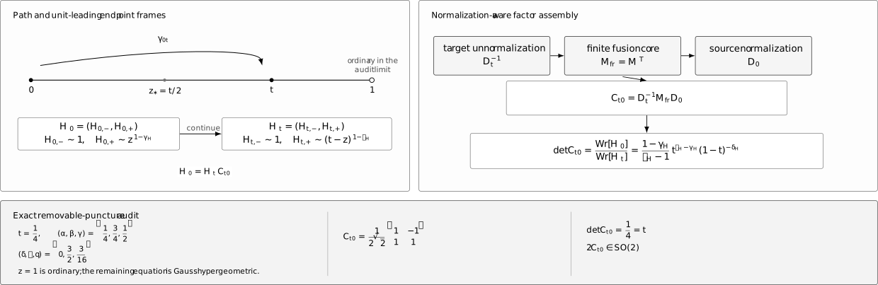
A path-labelled Heun connection matrix combines the finite fusion core $M_{\mathrm{fr}}$ with independent source and target normalizations. In the removable-$z=1$ audit, the equation reduces to a Gauss equation but the endpoint powers remain nontrivial; their assembly produces a scaled signed-Hadamard matrix whose determinant equals the Wronskian ratio.

Abel’s identity fixes the determinant

The gamma reflection formula gives

$$\det M_{\mathrm{fr}} = -\frac{a_0}{a_t} = \frac{ 1-\gamma_{\mathrm H} }{ \epsilon_{\mathrm H}-1 }.$$

The endpoint determinants give

$$\frac{ \det D_0 }{ \det D_t } = t^{\epsilon_{\mathrm H}-\gamma_{\mathrm H}} (1-t)^{-\delta_{\mathrm H}}.$$

Therefore

$$\boxed{ \det C_{t0} = \frac{ 1-\gamma_{\mathrm H} }{ \epsilon_{\mathrm H}-1 } t^{\epsilon_{\mathrm H}-\gamma_{\mathrm H}} (1-t)^{-\delta_{\mathrm H}}. }$$

The same result follows directly from the ODE. On $0<z<t$, set

$$\mathscr A(z) := z^{-\gamma_{\mathrm H}} (1-z)^{-\delta_{\mathrm H}} (t-z)^{-\epsilon_{\mathrm H}}.$$

Unit-leading asymptotics and Abel’s identity give

$$\begin{aligned} \Wr \left[ H_{0,-},H_{0,+} \right] &= (1-\gamma_{\mathrm H}) t^{\epsilon_{\mathrm H}} \mathscr A(z), \\ \Wr \left[ H_{t,-},H_{t,+} \right] &= (\epsilon_{\mathrm H}-1) t^{\gamma_{\mathrm H}} (1-t)^{\delta_{\mathrm H}} \mathscr A(z). \end{aligned}$$

Since $\boldsymbol H_0=\boldsymbol H_tC_{t0}$, their ratio is exactly the displayed determinant.

The block derivatives cancel from the determinant. This is necessary: the determinant of a connection matrix is fixed entirely by the two local Wronskian normalizations. The classical block controls individual entries, not their Wronskian-constrained product difference.

Three cheap implementation tests

1. Evaluate both local frames at one ordinary matching point and solve $C_{t0}=\Phi_t^{-1}\Phi_0$.
2. Repeat at a second matching point; the matrix must be unchanged.
3. Compare its determinant with the boxed Wronskian ratio.

Passing only the third test does not prove the four entries are correct, but failing it proves that they are not.

An exact removable-puncture benchmark

Choose

$$\begin{gathered} t=\frac14, \qquad \alpha_{\mathrm H}=\frac14, \qquad \beta_{\mathrm H}=\frac34, \\ \gamma_{\mathrm H}=\frac12, \qquad \delta_{\mathrm H}=0, \qquad \epsilon_{\mathrm H}=\frac32, \qquad q_{\mathrm H}=\frac3{16}. \end{gathered}$$

Both sides of the Fuchs relation equal $2$. Moreover,

$$\delta_{\mathrm H}=0, \qquad q_{\mathrm H} = \alpha_{\mathrm H}\beta_{\mathrm H},$$

so the apparent pole at $z=1$ cancels. The equation becomes

$$y'' + \left( \frac1{2z} + \frac3{2(z-t)} \right)y' + \frac3{16z(z-t)}y = 0.$$

With $x=z/t$, this is

$$x(1-x)y_{xx} + \left( \frac12-2x \right)y_x - \frac3{16}y = 0,$$

the Gauss equation with parameters

$$\left( a_{\mathrm G},b_{\mathrm G},c_{\mathrm G} \right) = \left( \frac14,\frac34,\frac12 \right).$$

The unit-leading endpoint bases are

$$\begin{aligned} H_{0,-} &= {}_2F_1 \left( \frac14,\frac34; \frac12; \frac zt \right), \\ H_{0,+} &= z^{1/2} {}_2F_1 \left( \frac34,\frac54; \frac32; \frac zt \right), \end{aligned}$$

and

$$\begin{aligned} H_{t,-} &= {}_2F_1 \left( \frac14,\frac34; \frac32; 1-\frac zt \right), \\ H_{t,+} &= (t-z)^{-1/2} {}_2F_1 \left( \frac14,-\frac14; \frac12; 1-\frac zt \right). \end{aligned}$$

The centered data are

$$a_0=\frac14, \qquad a_t=-\frac14, \qquad a_1=\frac12, \qquad a_\infty=-\frac14, \qquad a=\pm\frac14.$$

Here the unit-leading classical block vanishes:

$$\widehat f=0.$$

One way to see this is that the fourth puncture has become removable. At level one, the factor $d+\delta_1-\delta_\infty$ already vanishes; the reduction makes the vanishing persist to all levels.

The three factors are

$$M_{\mathrm{fr}} = \begin{pmatrix} \dfrac1{2\sqrt2} & -\dfrac1{\sqrt2} \\ \dfrac1{\sqrt2} & \sqrt2 \end{pmatrix},$$

and

$$D_0 = \operatorname{diag} \left( \frac12,\frac14 \right), \qquad D_t = \operatorname{diag} \left( \frac12,1 \right).$$

Thus

$$\boxed{ C_{t0} = \frac1{2\sqrt2} \begin{pmatrix} 1&-1 \\ 1&1 \end{pmatrix}. }$$

Its determinant is

$$\det C_{t0} = \frac14 = t.$$

The Wronskians independently give

$$\begin{aligned} \Wr[\boldsymbol H_0] &= \frac1{16} z^{-1/2} (t-z)^{-3/2}, \\ \Wr[\boldsymbol H_t] &= \frac14 z^{-1/2} (t-z)^{-3/2}, \end{aligned}$$

so their ratio is again $1/4$.

This example also separates unit-leading from equal-Wronskian normalization. Rescale only the zero frame:

$$\widetilde{\boldsymbol H}_0 := t^{-1/2}\boldsymbol H_0.$$

Then

$$\widetilde C_{t0} = t^{-1/2}C_{t0} = \frac1{\sqrt2} \begin{pmatrix} 1&-1 \\ 1&1 \end{pmatrix}, \qquad \widetilde C_{t0}\in SO(2).$$

The orthogonal matrix is attractive, but it belongs to a different endpoint normalization. The unit-leading matrix is the boxed matrix above.

A genuinely four-singular numerical audit

Return to the rational branch from the previous page:

$$\theta_0=\theta_t=\frac13, \qquad \theta_1=\theta_\infty=\frac15, \qquad \theta_{0t}=\frac35.$$

The standard-Heun parameters are

$$\begin{aligned} \gamma_{\mathrm H} &= \epsilon_{\mathrm H} = \frac23, & \delta_{\mathrm H} &= \frac45, \\ \alpha_{\mathrm H} &= \frac23, & \beta_{\mathrm H} &= \frac7{15}, \qquad a=\frac3{10}. \end{aligned}$$

Through level two,

$$\begin{aligned} q_{\mathrm H}^{[2]}(t) &= -\frac{14}{225} + \frac{14}{75}t + \frac{119}{5850}t^2, \\ F_0^{[2]}(t) &= \frac16t + \frac{11}{156}t^2, \\ F_t^{[2]}(t) &= -\frac16t - \frac5{52}t^2. \end{aligned}$$

At $t=0.04$, direct Frobenius evaluation of both local frames at $z=t/2$ gives

$$C_{t0}^{\mathrm{Frob}} \approx \begin{pmatrix} 0.6852083269 & 0.5321827959 \\ 1.0471097736 & -0.6945959089 \end{pmatrix}.$$

The level-two block formula gives

$$C_{t0}^{[2]} \approx \begin{pmatrix} 0.6852142054 & 0.5321841143 \\ 1.0470983914 & -0.6945967755 \end{pmatrix}.$$

The maximum entrywise relative error is $1.09\times10^{-5}$. Both determinants equal, to the shown working precision,

$$-1.033196707586\ldots,$$

because the determinant identity is independent of the block truncation.

Let order $N$ mean that $q_{\mathrm H}$ and $F_0,F_t$ are all truncated consistently through $t^N$. The direct Frobenius comparison is:

$t$	$N=0$	$N=1$	$N=2$
$0.08$	$1.84\times10^{-1}$	$2.16\times10^{-3}$	$9.12\times10^{-5}$
$0.04$	$1.00\times10^{-1}$	$5.19\times10^{-4}$	$1.09\times10^{-5}$
$0.02$	$5.23\times10^{-2}$	$1.27\times10^{-4}$	$1.33\times10^{-6}$
$0.01$	$2.68\times10^{-2}$	$3.15\times10^{-5}$	$1.64\times10^{-7}$

The columns scale respectively as $O(t)$, $O(t^2)$, and $O(t^3)$. This is the expected behavior of a consistently truncated formal connection formula away from poles and zeros of its entries.

The complete calculation, including the Heun recurrence, both frames, the block formula, and the determinant audit, is available as general-heun-connection-check.py. Because it fixes $z_*=t/2$, the script restricts this local-series audit to $0<t<2/3$, where the matching point lies in both Frobenius convergence disks.

Other endpoint pairs require transformed channel data

The displayed matrix is local to the small-$t$ $0t$ channel. Other adjacent pairs follow from Möbius transformations and permutations of the four punctures, but the transformation must act on all of the following:

1. the Heun parameters and accessory;
2. the local coordinates and their branch constants;
3. the external exponent lifts;
4. the classical block channel;
5. the source and target normalization matrices.

A nonadjacent connection, such as zero to infinity, can be factored through the intermediate annulus. At the semiclassical-block level its sign kernel, for $\theta,\theta'\in\{-1,+1\}$, has the form

$$\begin{aligned} \mathcal K_{\theta\theta'} ={}& \sum_{\sigma=\pm1} \mathcal M_{\theta\sigma} \left( a_0,a;a_t \right) \\ &\times \mathcal M_{-\sigma,\theta'} \left( a,a_\infty;a_1 \right) t^{-\sigma a} \ee^{-\sigma\partial_a\widehat f/2}. \end{aligned}$$

The sum over $\sigma$ is the two-dimensional intermediate basis. The physical zero-to-infinity matrix additionally has the source and target diagonal normalizations and the phase selected for the powers at infinity. The displayed $\mathcal K_{\theta\theta'}$ array is source-first and target-second, so the book’s target-row frame matrix uses $\mathcal K^{\mathsf T}$ before those endpoint dressings are applied. This is the simplest place where $\partial_a\widehat f$ appears.

Thus “use a crossing matrix” is not a complete prescription. One must name the channel, the transformed block, both endpoint frames, and the path. The later page on full connection coefficients organizes those ingredients systematically.

Branch changes act by endpoint matrices

Suppose a new path changes the continued endpoint frames to

$$\boldsymbol H_0M_0, \qquad \boldsymbol H_tM_t.$$

Then

$$C_{t0}^{\mathrm{new}} = M_t^{-1} C_{t0} M_0.$$

For nonresonant local loops in the declared bases,

$$M_0 = \operatorname{diag} \left( 1,\ee^{4\pi\ii a_0} \right), \qquad M_t = \operatorname{diag} \left( 1,\ee^{4\pi\ii a_t} \right),$$

with the orientation at $t$ interpreted in its local coordinate. The same covariance law handles a mere normalization change:

$$\widetilde C_{t0} = N_t^{-1} C_{t0} N_0.$$

This is why connection entries are not monodromy invariants. The Wronskian determinant, zero loci associated with a specified boundary problem, and conjugacy-invariant monodromy data transform in controlled ways, but the four raw numbers depend on the chosen frames.

A reliable computation workflow

1. Lock the equation. Check the Fuchs relation and compute $a_0,a_t,a_1,a_\infty$.
2. Lock the branch. Declare local coordinates, logarithms, and a continuation path.
3. Choose or invert the channel. Relate $q_{\mathrm H}$ and $a$ with the full classical accessory formula.
4. Compute one block consistently. Evaluate $\widehat f$, $\partial_{a_0}\widehat f$, and $\partial_{a_t}\widehat f$ on the same lifted branch.
5. Evaluate the fusion core. Use the indexed $\mathcal M_{sr}$ formula before arranging it into a matrix.
6. Assemble by covariance. Form $D_t^{-1}M_{\mathrm{fr}}D_0$.
7. Audit independently. Compare with Wronskians and, when numerical values are needed, with direct Frobenius matching.
8. Only then transform paths or bases. Apply the two-sided covariance law explicitly.

Common pitfalls

Using the accessory derivative as the Heun parameter. $\partial_tf$ is a normal-form residue. The standard parameter $q_{\mathrm H}$ is its affine image and must be related to $a$ before the connection formula is evaluated.

Reading the fusion array as the row-frame matrix. In $\mathcal M_{sr}$, the first sign labels the source and the second the target. The book’s connection matrix has target rows and source columns, so $M_{\mathrm{fr}}=\mathcal M^{\mathsf T}$.

Dropping external derivatives. The classical accessory depends on $\partial_t\widehat f$, whereas normalized adjacent connection entries depend on $\partial_{a_0}\widehat f$ and $\partial_{a_t}\widehat f$. These derivatives answer different questions.

Mixing $t-z$ with $z-t$. Fractional powers differ by a path-dependent phase. Change the target basis diagonally and transform $C_{t0}$ two-sidedly.

Trusting a component formula without its determinant. Gamma arguments are easy to mistype. The exact Wronskian ratio is a normalization-sensitive checksum for the complete matrix.

Substituting resonant parameters directly. When $2a_0$ or $2a_t$ is integral, the unit-leading power basis may degenerate and gamma factors can diverge separately. Construct the logarithmic basis or take a correlated limit of the full matrix.

Exercises

1. Derive the four powers of t

Starting from $C_{t0}=D_t^{-1}M_{\mathrm{fr}}D_0$, derive the powers of $t$ multiplying the four gamma coefficients.

Solution

For target sign $r$ and source sign $s$, the ratio of diagonal powers is

$$\begin{aligned} \frac{ t^{\frac12-a_t+sa_0} }{ t^{\frac12-a_0+ra_t} } &= t^{ a_0(s+1)-a_t(r+1) }. \end{aligned}$$

For $(r,s)=(-,-),(-,+),(+,-),(+,+)$ this gives

$$1, \qquad t^{2a_0}, \qquad t^{-2a_t}, \qquad t^{2a_0-2a_t}.$$

Using $2a_0=1-\gamma_{\mathrm H}$ and $2a_t=1-\epsilon_{\mathrm H}$ gives

$$1, \qquad t^{1-\gamma_{\mathrm H}}, \qquad t^{\epsilon_{\mathrm H}-1}, \qquad t^{\epsilon_{\mathrm H}-\gamma_{\mathrm H}}.$$

2. Prove the fusion-core determinant

Show that

$$\det M_{\mathrm{fr}} = -\frac{a_0}{a_t}.$$

Solution

Since transposition does not change a determinant, compute the determinant of the array $\mathcal M_{sr}$. Factor

$$\Gamma(1-2a_0) \Gamma(1+2a_0) \Gamma(2a_t) \Gamma(-2a_t)$$

from the two products. Apply

$$\Gamma(1+x)\Gamma(1-x) = \frac{\pi x}{\sin\pi x}$$

to the $a_0$ pair. For the $a_t$ pair, first use the recurrence

$$\Gamma(1-x) = -x\Gamma(-x)$$

to obtain

$$\Gamma(x)\Gamma(-x) = -\frac{\pi}{x\sin\pi x}.$$

For complementary denominator pairs use

$$\Gamma(x)\Gamma(1-x) = \frac{\pi}{\sin\pi x}$$

to complementary denominator pairs. The remaining difference of sine products reduces by

$$\sin(u+v)\sin(u-v) = \sin^2u-\sin^2v.$$

All dependence on the internal lift $a$ cancels, leaving

$$\det M_{\mathrm{fr}} = -\frac{a_0}{a_t}.$$

The cancellation of $a$ is required because the determinant is fixed by endpoint Wronskians.

3. Catch the lower-right gamma inconsistency

Use only the sign-indexed fusion formula to find the numerator of $\mathcal M_{++}$. Explain why $\Gamma(\epsilon_{\mathrm H}-1)\Gamma(\gamma_{\mathrm H})$ cannot be correct generically.

Solution

Set $s=r=+1$:

$$\Gamma(-2a_t) \Gamma(1+2a_0) = \Gamma(\epsilon_{\mathrm H}-1) \Gamma(2-\gamma_{\mathrm H}).$$

Replacing the second factor by $\Gamma(\gamma_{\mathrm H})$ treats the $s=+$ source branch as if it carried $1-2a_0$ rather than $1+2a_0$. It also destroys

$$\det M_{\mathrm{fr}} = -\frac{a_0}{a_t},$$

and hence fails the Abel–Wronskian determinant check.

4. Change the target local coordinate

On an upper-half-plane continuation, replace the target power $(t-z)^{2a_t}$ by $(z-t)^{2a_t}$. Find the new connection matrix.

Solution

On that continuation,

$$(z-t)^{2a_t} = \ee^{2\pi\ii a_t} (t-z)^{2a_t}.$$

Thus

$$\widetilde{\boldsymbol H}_t = \boldsymbol H_t \operatorname{diag} \left( 1,\ee^{2\pi\ii a_t} \right).$$

The source frame is unchanged, so

$$\widetilde C_{t0} = \operatorname{diag} \left( 1,\ee^{-2\pi\ii a_t} \right) C_{t0}.$$

A lower-half-plane continuation replaces the phase by its inverse.

5. Reproduce the radical benchmark

For the removable-puncture parameters, multiply the three displayed factors and check the determinant.

Solution

Direct multiplication gives

$$\begin{aligned} D_t^{-1}M_{\mathrm{fr}}D_0 &= \begin{pmatrix} 2&0\\ 0&1 \end{pmatrix} \begin{pmatrix} \dfrac1{2\sqrt2} & -\dfrac1{\sqrt2} \\ \dfrac1{\sqrt2} & \sqrt2 \end{pmatrix} \begin{pmatrix} \frac12&0\\ 0&\frac14 \end{pmatrix} \\ &= \frac1{2\sqrt2} \begin{pmatrix} 1&-1\\ 1&1 \end{pmatrix}. \end{aligned}$$

Therefore

$$\det C_{t0} = \frac18 \left[ 1-(-1) \right] = \frac14.$$

The general determinant formula gives

$$\frac{ 1-\gamma_{\mathrm H} }{ \epsilon_{\mathrm H}-1 } t^{\epsilon_{\mathrm H}-\gamma_{\mathrm H}} = \frac{1/2}{1/2} \left( \frac14 \right)^1 = \frac14,$$

because $\delta_{\mathrm H}=0$.

6. Show invariance under the internal sign

Prove that the adjacent matrix is unchanged by $a\mapsto-a$.

Solution

Each fusion coefficient contains the symmetric denominator product

$$\Gamma(X+a)\Gamma(X-a),$$

so $\mathcal M_{sr}$ is even in $a$. The four-point classical block depends on the internal classical weight

$$d=\frac14-a^2$$

and is likewise even on the sign-paired lift. Hence $F_0$, $F_t$, $D_0$, and $D_t$ are unchanged. Every factor in

$$C_{t0} = D_t^{-1}M_{\mathrm{fr}}D_0$$

is therefore invariant.

This does not erase the lifted channel label: nonadjacent factorizations contain a sum over intermediate signs and factors such as $t^{-\sigma a}\ee^{-\sigma\partial_a\widehat f/2}$.

7. Predict the truncation error

Suppose $\widehat f$ is known through $t^N$ and the accessory relation is truncated consistently. What generic relative accuracy should the matrix have as $t\to0$?

Solution

The omitted block tail begins at $t^{N+1}$. Its external derivatives also begin at that order. The accessory relation determined from the same truncated block gives $a(q_{\mathrm H},t)$ through the corresponding order, provided the local inversion is nondegenerate. Taylor expansion of the gamma and exponential factors then gives

$$\frac{ (C_{t0}^{[N]})_{rs} -(C_{t0})_{rs} }{ (C_{t0})_{rs} } = O(t^{N+1})$$

for each fixed entry $(r,s)$, away from its zeros or poles. This predicts the $t$, $t^2$, and $t^3$ columns in the numerical table.

8. Turn a boundary condition into a scalar equation

Suppose the desired solution is the ordinary branch $H_{0,-}$ at zero and must be proportional to the raised branch $H_{t,+}$ at $t$. Which connection entry must vanish?

Solution

The first column of

$$\boldsymbol H_0 = \boldsymbol H_tC_{t0}$$

is

$$H_{0,-} = (C_{t0})_{--}H_{t,-} + (C_{t0})_{+,-}H_{t,+}.$$

For $H_{0,-}$ to contain no ordinary target branch, one needs

$$(C_{t0})_{--}=0.$$

In the displayed formula this is a zero of

$$\mathcal M_{--} \ee^{(F_t-F_0)/2}.$$

The exponential never vanishes on a regular branch, so the condition is encoded by a reciprocal-gamma zero, subject to the accessory relation that ties $a$ to $q_{\mathrm H}$.

References

• NIST Digital Library of Mathematical Functions, §31.2, “Differential Equations” and §31.3, “Basic Solutions”. These sections fix the standard Heun equation, local recurrences, and transformed Frobenius germs.
• G. Bonelli, C. Iossa, D. Panea Lichtig, and A. Tanzini, “Irregular Liouville Correlators and Connection Formulae for Heun Functions”, Communications in Mathematical Physics 397 (2023), 635–727; arXiv:2201.04491. Section 3.1, especially equations (3.1.30) and (3.1.35), gives the semiclassical adjacent and nonadjacent block relations. Section 4.1, equations (4.1.15)–(4.1.22), translates them to Heun coefficients; Appendix C.1 gives the block and accessory expansion.
• O. Lisovyy and A. Naidiuk, “Perturbative Connection Formulas for Heun Equations”, Journal of Physics A: Mathematical and Theoretical 55 (2022), 434005; arXiv:2208.01604. Corollary 3.2 gives the Schäfke–Schmidt large-order connection formula, and Theorem B gives an exact continued-fraction representation in its stated domain. Their ordinary-Heun comparison checks the classical-block formula through order $\lambda^3$; it is not a global proof of that formula.
• M. Piątek and A. R. Pietrykowski, “Solving Heun’s Equation Using Conformal Blocks”, Nuclear Physics B 938 (2019), 543–570; arXiv:1708.06135. This work develops the heavy–light factorization and Floquet-type Heun solutions behind the classical construction.