Method Selection and Open Research Problems

The safest first method for a new black-hole ODE is not the most elaborate one. It is the method that computes the requested physical datum with the fewest unproved identifications. A continued fraction may be ideal for QNM locations but insufficient for a normalized residue. A Painlevé tau function may reconstruct an accessory but not select the endpoint flag. An exact-WKB period may encode a boundary coefficient in one Stokes chamber but not after an untracked graph mutation. A holographic connection quotient is not a correlator until the variational and counterterm ledger is restored.

The Chapter 14 capstones selected methods from operator domains and turning-point topology. Black-hole problems add three nonoptional layers: causally selected horizon lines, angular or matrix closure, and observable normalization.

This page turns those distinctions into a working decision procedure. It then uses the failed gates themselves to define research problems. “Open” means that a normalization-complete result with the stated scope is not supplied by the cited literature as of July 2026; it does not mean that no partial result, formal construction, or numerical evidence exists.

First reading

Choose the requested output in the first table, follow the universal spine, and apply only the method gates that can be proved for the named operator. Read the frontier section when planning a new project rather than solving a known benchmark.

Status discipline

Label	Minimum evidence
Exact	The analytic statement follows on the declared chart with every branch, normalization, and existence hypothesis satisfied
Controlled	A limit or truncation has an explicit small parameter or refinement axis, a stated domain, and a remainder or error estimate that improves along it
Conditional	A named analytic hypothesis—such as Borel summability, Stokes topology, endpoint continuation, or zero-free strip—remains to be proved
Conjectural	The physical identification itself is proposed and supported but not derived
Numerical	Finite-precision evidence with reproducible controls; not an existence or completeness theorem

The requested output determines the minimum data

Before classifying singularities, decide what the calculation must return. The same radial ODE supports questions with different normalization and global requirements.

Spectra and amplitudes.

Requested output	Minimum analytic object	Additional ledger that cannot be omitted
QNM locations	Boundary Wronskian, Evans/Jost function, recurrence boundary function, or source determinant	Time convention, endpoint lines, angular sheet, frequency sheet, and exceptional strata
Multiplicity or exceptional point	Analytic scalar boundary function or full source matrix near the root	Argument-principle count, kernel dimension, partial multiplicities, crossing matrix, or Jordan chain
Reflection, transmission, or greybody factor	Relevant entries of a full connection matrix	Same-endpoint Wronskians, flux normalization, field reconstruction, and real-frequency continuation
QNM residue or excitation coefficient	Normalized numerator and derivative of the boundary function	Endpoint amplitudes, bilinear pairing or Green-function normalization, and contour prescription
Static response or Love number	Zero-frequency growing/decaying coefficient ratio	Static endpoint basis, field reconstruction, gauge-invariant observable, and subtraction convention

Observables and singular limits.

Requested output	Minimum analytic object	Additional ledger that cannot be omitted
Retarded AdS correlator	Source and response matrices plus renormalized canonical momentum	Bulk action, scalar or matrix gauge, counterterms, finite scheme, and boundary quantization
Pole-skipping	Two-parameter horizon and boundary source maps	Rank loss, transverse unfolding, observable projection, and limiting direction
Time-domain response	Meromorphically or branchwise continued resolvent	QNM poles and residues, branch cuts, large-frequency arcs, prompt term, and contour deformation

For generic QNM locations and multiplicities, multiplying the boundary function by a holomorphic unit is harmless. A physical residue is preserved only if the accompanying numerator and normalization transform consistently. A pole table also does not determine a time-domain signal when branch cuts or high-frequency contours contribute.

For a separated rotating problem, keep

$$\mathcal F(A,\omega) = \begin{pmatrix} E_{\mathrm{ang}}(A,\omega) \\ E_{\mathrm{rad}}(A,\omega) \end{pmatrix}$$

until a regular angular graph $A(\omega)$ has actually been proved. For coupled bulk fields, replace this two-component scalar map by the source matrix $\mathsf A(\omega,k)$; taking its determinant too early can hide kernel dimension and observable projections.

The direct boundary problem is the universal spine

Every route begins with the same five steps.

1. Freeze the physical operator. Record the Fourier sign, separated field variable, radial and angular domains, background stratum, and parameter units.
2. Derive the local flags. Use regular horizon coordinates, declared AdS boundary conditions, causal flat-infinity continuation, and regular angular axes. Declare the generic normalizations and rebuild them on singular strata.
3. Construct the primary global function. Use a weighted Wronskian, selected connection entry, or source matrix whose zero has the intended physical meaning.
4. Run the exceptional-stratum stop test. Check exponent resonances, thresholds, synchronous frequencies, angular branch points, and extremality before selecting a generic engine.
5. Build a direct evaluation. Match Frobenius or sectorial solutions, derive a recurrence with its minimal-line transfer, integrate a Riccati equation, or use collocation in the original variables. Add recurrence-coefficient zeros, minimality walls, and Stokes mutations to the exceptional map as they arise.

Only then ask whether an extra representation reduces cost or reveals new analytic structure. The direct function remains the control even when the modern route is more efficient.

Completeness inside a declared contour requires the argument-principle count and multiplicity audit from Page 7. Remove poles introduced by a meromorphic normalization, or count zeros minus poles rather than interpreting a candidate list as complete.

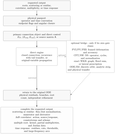
The boundary invariant and a direct engine form the solid spine. A tau function, quantum period, Voros symbol, or $Q$-function is an optional bridge admitted only after its own gate closes. The last box adds the normalization or dynamical data required by the requested output.

Add a representation only after its gate closes

The following order minimizes assumptions. It is not a ranking of mathematical sophistication.

Direct engines.

Engine	Minimum prerequisite	Native output
Closed special-function connection	Exact operator/gauge map and valid parameter chart	Normalized connection entries when endpoint factors are retained
Direct Wronskian, Riccati matching, or collocation	Constructible physical endpoint frames and a continuation domain	Boundary divisor; amplitudes only with normalized frames
Recurrence or continued fraction	Exact synthesis, homogeneous seed, large-order branches, and minimal-tail transfer	Efficient divisor chart; not automatically a connection amplitude

Conditional bridges and output completion.

Bridge	Fast admission test	Native output and remaining gap
PVI/PV or conformal blocks	Explicit deformation/scalarization, accessory relation, exponent lifts, and framed endpoint flag	Tau/monodromy representation; a trace or tau zero alone is not spectral
PIII-type inverse problem	Explicit rank-two lift, wild framing, scalar slice, and normalized confluence/accessory map	Two-irregular monodromy data; a generic DCHE does not license PIII
CFT/SW/NS	Ordered quantum operator, masses, $U(1)$ scheme, cycles, logarithm lift, Matone branch, and nonzero prefactor	Quantum periods or connection coefficient; a matching curve is insufficient
Exact WKB	Formal $\hbar$, sheet, graph, Stokes word, cycle, existence and Borel/lateral prescription, and transfer to the physical line	Voros symbols and connection word; graph walls require mutation
ODE/IM or TBA	Discrete orbit of normalized canonical solutions, physical endpoint continuation, strip, divisor, and asymptotic data	Canonical $Q$ or integral equations; two irregular ends do not suffice
Holographic renormalization	Variational problem, physical radial powers, source/response gauge, counterterms, and finite scheme	Fully normalized $G_{\mathrm R}$; it completes rather than replaces the ODE solve

Several methods may pass their gates simultaneously, as in generic Kerr. Use one as the primary computation and the most independent other route as the audit. Do not average two outputs that disagree before locating the mismatched branch, gauge, or boundary flag. Every admitted bridge must return to the physical Wronskian or source map, and its refinement parameter must be varied independently of the direct lane.

Exceptional strata override the ordinary choice

A familiar method can become the wrong method at a special parameter value. The correct response is usually to rebuild the analytic chart, not merely to increase precision. The preceding singular-phenomena page derives the local distinctions. Four stop categories suffice for selection:

• Local-basis degeneration. At coincident exponents, an integral gap with nonzero Frobenius obstruction, a BF coalescence, $\omega=0$ at flat infinity, or a synchronous horizon frequency, the generic power or wave-normalized chart can coalesce, become singular, or become integrally resonant. Inspect the obstruction and use a static, Levelt, or logarithmic frame only when the local equation requires it.
• Confluence or sector mutation. At extremality, a Stokes wall, or an ODE/IM divisor entering the analytic strip, rebuild the sectorial solutions, graph/cycles, or excited-state contour before continuing a generic formula.
• Analytic chart failure. At an angular branch point, recurrence pivot or minimality wall, or block/Matone/Gamma divisor, retain the full zero germ and change coordinates, homogeneous recurrence, or analytic channel.
• Rank loss. At pole-skipping the horizon recurrence loses rank and the ingoing solution space gains an additional free datum. Use the full two-parameter source/response map and compute its directional unfolding.

Confluence deserves special caution. The limit

$$\text{regular horizons} \longrightarrow \text{extremal irregular horizon}$$

changes the local category. Taking a subextremal formula at fixed overtone, fixed horizon-frame frequency, or fixed boundary frequency can give different limits. Declare which variables are held fixed and compare the limiting connection matrix, not only a list of roots.

Two checks must have different failure modes

The strongest practical certificate combines a structural identity with two numerical lanes whose dominant errors are not shared.

Primary lane	Weak “second check”	Genuinely useful second check
Continued fraction	Same fraction at a larger depth	Original-variable Riccati matching or collocation
PVI/PV tau expansion	More terms in the same channel	Selected Heun Wronskian with independently continued endpoint bases
Finite NS instanton series	A different optimizer on the same truncation	Direct angular and radial residuals; vary instanton order and ODE precision independently
Borel–Padé Voros symbol	Another Padé shape using the same coefficients	Direct boundary Wronskian or a separately derived recurrence
ODE/IM TBA	QQ identity reconstructed from the same TBA solution	Direct canonical Wronskian and, separately, the physical endpoint Wronskian
Pseudospectral discretization	A denser grid in the same coordinate	Wronskian/recurrence calculation with different endpoint treatment

At a candidate $(A_*,\omega_*)$, report scaled residuals for every physical component, the coupled Jacobian or local multiplicity data, and the change under each refinement axis. Near a nonnormal spectral problem, eigenvalue agreement should be supplemented by condition numbers or pseudospectral information; many digits in a root do not imply dynamical robustness.

A useful negative control deliberately crosses a gate. Move through a recurrence minimality wall, detune a discrete ODE/IM symmetry, cross a Stokes wall without mutating the graph, or omit the angular equation. The computation should fail or reorganize in the way predicted by its hypotheses. If it does not, the implementation is probably insensitive to the structure it claims to use.

Keep a four-layer publication record

The Page 8 capstone gives the full cross-method comparison certificate. For choosing and reporting a method, its content can be compressed into four layers:

1. Invariant: the original operator, physical endpoint flags, angular or matrix closure, and boundary function.
2. Engine: the canonical crosswalk, admitted method gate, chart, branches, excluded divisors, and status label.
3. Output completion: multiplicity data, normalized numerator and residue, holographic action data, or cut discontinuity—whichever the requested claim needs.
4. Audit: original-variable residuals, an independent representation, separate refinement axes, a negative control, and machine-readable precision and truncation data.

Open problems are missing arrows

A broad label such as “solve Kerr” or “apply ODE/IM to black holes” is not yet a research problem. A useful problem names three things: the strongest map already established, the arrow that is missing at the intended normalization grade, and an observable test that could falsify the proposed completion. The programs below use that standard. Their status was checked against the primary literature through 25 July 2026.

Physical determinant atlas

Established. Conformal-block and instanton constructions give generic-chart formulas for Heun and confluent-Heun connection coefficients, with the all-orders and general-endpoint status qualifications stated in Chapter 7. Rigorous Kerr frameworks independently define QNMs as resolvent poles or generator eigenvalues, and generic Kerr has a successful PV inverse-monodromy formulation. For strict-extremal Reissner–Nordström, the SW/NS column now supplements the exact-WKB entry: Wang, Yang, and Zhang give an exact DCHE–$SU(2)$, $N_f=2$ operator dictionary and charged-massive scalar spectra in the July 2026 version of their work.

Missing arrow. There is no general normalization-complete theorem that identifies a physically normalized endpoint Wronskian with the relevant tau function, NS period, $Q$-function, or resummed Voros symbol on a stated covering domain. The remaining strict-extremal RN question is therefore not whether an SW dictionary exists. It is whether the selected B-period branch is the physical ingoing/outgoing Wronskian up to a holomorphic unit, with controlled instanton continuation and independent checks in the new charged-massive sector.

Decisive milestone. Construct physical endpoint frames and prove

$$D_{\mathrm{modern}}(\omega,\lambda) = u(\omega,\lambda)E_B(\omega,\lambda), \qquad u\in\mathcal O^\times(U),$$

on an explicit sheet $U$. Give overlap functions between charts and new Levelt, sectorial, or confluent charts at every excluded divisor. Equality of zero orders and the transformation of residues must be part of the theorem.

Coupled Kerr–Newman

Established. Scalar Kerr–Newman separates. The physical electromagnetic and gravitational perturbations instead form a gauge-invariant coupled system of two PDEs and are not known to separate generically. Slow-rotation and near-horizon expansions, as well as direct two-dimensional numerics, already resolve important spectra and eigenvalue repulsions. This marks a present boundary of the chapter’s ODE workflow: generic separation of the full coupled system has not been established. The separable Dudley–Finley equation is a decoupled spin-weighted approximation, not the full Einstein–Maxwell system.

Missing arrow. Scalar Heun, PV, SW, or exact-WKB formulas do not provide a matrix connection object for the coupled fields. Nor do they determine whether the observed repulsions are organized by exceptional points in complexified parameter space or, at an actual degeneracy, supply algebraic multiplicity and Jordan data.

Decisive milestone. Either prove a true generic separation or construct a gauge-invariant matrix Evans/source map for the coupled PDE. Its zero set should agree with independently converged two-dimensional numerics and its local Weierstrass data and Fitting ideals should distinguish crossings, avoided crossings, and exceptional points throughout spin, charge, and extremality. Smith data may be used on declared one-parameter slices.

Uniform extremal connection limit

Established. PV/PIII confluence, near-horizon matching, rigorous estimates for the $\mathcal O(\kappa)$ scalar spectrum of near-extremal RN–dS, strict-extremal SW/NS, and strict-extremal exact WKB each control part of the problem. Extremal Kerr Green functions have separately been analyzed at both the zero-frequency and superradiant-bound branch points.

Missing arrow. No single connection construction is uniform in horizon separation, unscaled frequency, and the scaled frequency $\omega/T$. It must keep damped and zero-damped families distinct and explain when a nonuniform pole lattice converges to a branch-cut discontinuity. The limits

$$\begin{aligned} \kappa&\to0 &&\text{at fixed }\omega,\\ \kappa&\to0 &&\text{at fixed }(\omega-m\Omega_H)/\kappa \end{aligned}$$

are different analytic questions.

Decisive milestone. Derive a normalized connection matrix with a uniform remainder across CHE-to-DCHE and PV-to-PIII confluence. It should recover both mode families, select the physical branch without continuation from a known root, and converge in a specified sense to the limiting resolvent discontinuity.

Exact-WKB chamber atlas

Established. The Schwarzschild analysis of Miyachi and collaborators incorporates logarithmic Stokes spirals and horizon branch cuts that a naive finite turning-point diagram misses. Hatsuda and Shiga obtain high-precision scalar QNMs for extremal RN and selected extremal Kerr sectors from long WKB series and Borel–Padé resummation. A separate 2026 study treats the high-overtone limit for a class of parametrized nonextremal black holes.

Missing arrow. The physical parameter space is not yet covered by a proved Stokes-graph atlas. Present results leave topology assumptions, turning-point connections, summability, and error bounds only partially controlled. Hatsuda and Shiga’s scalar Kerr calculation excludes the exceptional $m=\ell=2$ Stokes geometry; uniform physical chamber control for extremal Kerr, higher spins, and normalized scattering or excitation data remains incomplete.

Decisive milestone. Classify graph chambers and mutations, including logarithmic spirals and turning-point collisions; prove Borel summability or declare controlled lateral sums in each chamber; and bound the resummation error in the physical connection coefficient rather than only observe stable digits in its zeros.

Physical ODE/IM beyond the fundamental strip

Established. The D3 modified-Mathieu problem has a discrete orbit of normalized subdominant solutions, exact QQ/TQ relations, Bethe-root conditions, and a ground-state TBA. Related $SU(2)$ matter systems extend the integrable structure to $N_f=1,2$. These achievements rely on special canonical rotations, not merely on having two irregular singularities.

Missing arrow. The D3 TBA is initially valid in a fundamental strip; other overtones require excited-state continuation. For residues and scattering observables, an explicit nonzero factor relating the canonical $Q$ to the physically normalized throat/infinity Wronskian remains required. No structural classification of which black-hole DCHEs possess a closed canonical orbit is supplied by the cited works.

Decisive milestone. Derive the excited-state source terms and contour deformations in every relevant strip, prove overtone enumeration, and show that the continued $Q$ equals the physical boundary function up to a nowhere-zero analytic factor. A classification theorem should reject a symmetry-free DCHE rather than manufacture a QQ relation from its singularity type.

Holographic correlators beyond scalar Heun charts

Established. Scalar four-singularity problems admit accurate recurrence connection quotients. In planar RN–AdS$_5$, a controlled low-temperature double scaling follows pole condensation into the zero-temperature cut. Scalar logarithmic Frobenius limits are available. For pole-skipping, local coupled-field matrix criteria that require no master variable and a high-order near-extremal scalar hierarchy now exist.

Missing arrow. A quotient known only up to a prefactor locates poles only on charts where that prefactor is proved to be a nowhere-zero holomorphic unit; it does not fix residues, contact terms, or transport normalization. Within the recurrence/conformal-block connection program considered here, normalization-complete logarithmic and coupled source/response matrices, action-level counterterms, continuation beyond the controlled low-temperature fixed-$\omega/T$ chart, holographic confluent-Heun recurrence quotients, and equations with more than four singularities remain incomplete. At pole-skipping, local horizon rank loss does not by itself prove a global numerator–denominator intersection.

Decisive milestone. Return a renormalized matrix correlator

$$G_{\mathrm R} = \mathsf M\mathsf B\mathsf A^{-1} + \mathsf P_{\mathrm{loc}},$$

with its bulk-action normalization, Ward identities, contact scheme, continuation beyond the controlled low-temperature chart, and a two-variable normal form at each rank defect. Direct radial integration must reproduce poles, zeros, residues, and directional pole-skipping limits.

Multiple zeros and operator dynamics

Established. A massive-scalar Kerr exceptional point has been found by isomonodromic methods, and recent resonance studies display the expected two-sheeted Puiseux geometry and polynomially enhanced time signal in controlled models. Kerr also possesses a conserved bilinear form that can normalize excitation coefficients for separated Teukolsky QNMs.

Missing arrow. When a connection calculation encounters a repeated scalar zero, it usually does not yet prove that its order equals the algebraic multiplicity of the full evolution generator, compute the geometric multiplicity, or construct generalized resonant states. Those distinctions are indispensable at actual Kerr–Newman or holographic degeneracies. Related but different source-map rank data are required at pole-skipping.

Decisive milestone. Relate the partial multiplicities of the analytic source map to the rank and order of the resolvent pole. Construct the Jordan chain and Puiseux monodromy and verify the predicted $t^j e^{-\ii\omega_*t}$ terms in a physical time-domain evolution.

Causal reconstruction beyond pole tables

Established. Rigorous subextremal Kerr frameworks now define resonances through meromorphic resolvents or hyperboloidal generators. Separate analyses derive selected branch-point asymptotics, tail terms, resonant expansions, and QNM excitation coefficients in particular settings.

Missing arrow. A finite or even complete list of poles in one meromorphic sector does not supply the prompt term, cut discontinuities, threshold behavior, or large-frequency arcs. It also does not establish that a QNM sum is complete in the function space of the initial-value problem.

Decisive milestone. Construct one sheet-aware spectral object whose zeros, normalized residues, cut jumps, and high-frequency estimates justify a causal contour deformation with a controlled remainder. The construction must remain meaningful in the extremal limit where pole families can condense into cuts.

Certified spectra and conditioning

Established. Continued fractions, PV tau expansions, NS instanton sums, Borel–Padé calculations, recurrence quotients, collocation, and complex scaling often agree to many digits. Black-hole pseudospectral studies also show that some overtones are strongly nonnormal and spectrally sensitive.

Missing arrow. Cross-method agreement is not an interval-certified proof of existence, uniqueness, multiplicity, or completeness. Arbitrary precision does not bound a recurrence tail, a Fredholm truncation, a resummation error, or the distance to a nearby multiple root.

Decisive milestone. Combine ball or interval evaluation of the boundary function with argument-principle counts, validated continuation, certified tail and resummation bounds, and reported condition numbers or pseudospectra. A successful computation should enclose every root inside a declared bounded contour or domain, prove the total multiplicity there, and distinguish numerical uncertainty from physical spectral sensitivity.

How to scope a viable project

Choose one missing arrow on one explicit parameter sheet. State which unit, residue, or matrix data must be recovered, name a direct original-ODE baseline, and specify a failure test before calculating. “Agreement for the first ten modes” is evidence; “the enclosed boundary functions have the same divisor and normalized derivative on $U$” is a completion claim.

Common pitfalls

Choosing a solver before choosing the output. A fast root solver may be excellent and still be incapable of returning a residue or a normalized correlator. Start from the first table and work backward to the minimum analytic object.

Treating two descendants of one identity as independent checks. A tau series, its conformal-block expansion, and an NS expression derived through the same connection formula can share every decisive convention error. Pair one of them with an original-variable Wronskian, collocation, or a recurrence derived independently.

Calling a singularity class a method license. Four regular singularities do not select a framed PVI boundary flag, and two irregular singularities do not create a discrete ODE/IM orbit. Check the deformation, framing, symmetry, analyticity, and continuation gates separately.

Interpreting “not established here” as impossibility. A conditional or open label records the missing proof at the stated scope and cutoff. It does not rule out a narrower theorem, a later result, or an alternative representation.

Calling a root list a dynamical prediction. Time-domain response depends on normalized residues, cuts, thresholds, arcs, and the initial-data projection. Pole locations alone describe only one part of that contour decomposition.

Exercises

1. Escalate a continued-fraction claim

A three-term continued fraction converges to a complex frequency to 40 digits. List the additional work required to claim, in succession: (a) a QNM frequency, (b) its Green-function residue, and (c) a fully normalized holographic retarded correlator.

Solution

For (a), derive the recurrence from the physical local solution, prove which large-order branch is minimal, transfer that branch to the intended remote endpoint, close the angular problem if present, state the frequency sheet, and check the zero with an original-variable boundary function. Forty stable digits in a ratio recursion do not supply those identifications.

For (b), retain the normalized numerator and differentiate the analytic boundary map on the same sheet. One also needs the appropriate Wronskian or bilinear normalization and the projection onto the physical field. A holomorphic-unit rescaling of the denominator without the corresponding numerator transformation changes the reported residue.

For (c), identify the nonnormalizable and normalizable coefficients in the physical radial gauge, derive the canonical momentum from the bulk action, add divergent counterterms, declare the finite scheme and quantization, and form the complete source/response matrix if fields mix. Ward identities and an independent direct solve then audit the result.

2. Route four operator passports

For each case, name the direct baseline, one optional bridge that is licensed only after extra proof, and one tempting but unjustified shortcut:

1. a generic confluent-Heun radial equation with two physical endpoint lines;
2. a framed four-regular-singularity family with a true modulus;
3. a symmetry-free doubly confluent equation with two irregular endpoints;
4. a resonant AdS system with a matrix source map.

Solution

1. Use a physical Wronskian, collocation, or a recurrence whose endpoint transfer has been proved. PV or SW/NS is optional only after the complete wild-monodromy or gauge-theory dictionary is fixed. “It is CHE” is not a quantization rule.
2. Use direct endpoint matching as control. PVI becomes available after an explicit isomonodromic deformation, accessory relation, exponent lifts, and framed boundary flag are supplied. A composite-monodromy trace alone is the tempting shortcut.
3. Use sectorial Wronskians or direct complex-contour integration. Exact WKB is optional after its graph, cycles, and summation direction are known. ODE/IM is unjustified without a discrete orbit of normalized canonical solutions.
4. Compute the resonant Frobenius obstruction; use a logarithmic Fefferman–Graham frame only when it is nonzero or the exponents coalesce. Propagate the full source and response matrices, then perform holographic renormalization. A generic scalar Gamma or Heun quotient, or an early reduction to $\det\mathsf A$, can lose mixing and rank data.

3. Audit independence

Five implementations are available: a PV Fredholm determinant, the $c=1$ block expansion of the same tau function, an NS series derived from the same connection identity, a Leaver recurrence, and original-variable collocation. Which pair gives the strongest independent spectral certificate? Which pairing directly audits the PV representation? State how the errors should be varied.

Solution

The Leaver recurrence and original-variable collocation are the cleanest spectral certificate because their representations, endpoint enforcement, and dominant truncation errors differ. Vary recurrence depth and collocation resolution or domain mapping independently, and evaluate both physical angular and radial residuals at the same candidate.

To audit the PV representation, pair the PV Fredholm determinant with either independent direct lane and compare the selected boundary function, not only the root. The block and stated NS implementations are not independent of PV when they inherit the same canonical dictionary and connection identity; they instead test convergence within that shared representation.

4. Apply the exceptional-stratum stop rule

Continue a Kerr mode toward both $r_+-r_-\to0$ and $\omega-m\Omega_H\to0$. Explain which parts of a generic subextremal calculation must be rederived before a limiting frequency is trusted.

Solution

As $r_+-r_-\to0$, the coordinate that sends the two horizons to separate regular singular points degenerates; the two local bases must be replaced by a sectorial irregular-horizon basis. A subextremal recurrence may lose its synthesis domain or minimal-tail interpretation, and the relevant Stokes graph and cycles can mutate.

As $\omega-m\Omega_H\to0$, the horizon exponents coalesce or become integer-resonant in the chosen horizon gauge, depending on the field variable and spin. One must construct the synchronous regular or Levelt/logarithmic frame selected by the local obstruction before dividing by exponent differences or Gamma factors. The two limits interact, so the calculation must declare whether the unscaled frequency or $(\omega-m\Omega_H)/\kappa$ is held fixed. Agreement of limiting root lists does not substitute for convergence of the normalized connection matrix.

5. State a research-grade equivalence theorem

A proposed black-hole $Q$-function and a direct boundary Wronskian have the same first 50 numerical zeros. State the additional hypotheses and conclusions needed for a local spectral-equivalence theorem.

Solution

Choose a connected parameter chart $U$ on an explicit spectral cover. Fix the operator gauge, physical endpoint frames, canonical $Q$ normalization, frequency sheet, continuation paths, and all excluded divisors. Prove both functions holomorphic on $U$ and prove

$$Q(\omega,\lambda) = u(\omega,\lambda)E_B(\omega,\lambda), \qquad u\in\mathcal O^\times(U).$$

This identifies the complete divisor with multiplicity, not merely 50 sample zeros. If residues are claimed, determine $u$ rather than only proving it is nonzero. Supply transition functions at adjacent charts and an independent original-ODE validation with certified root counts. A mismatch at a resonant or confluent divisor is not covered unless a replacement chart and its limit are part of the theorem.

6. Design a falsifiable frontier project

Choose the problem “normalize a recurrence-derived finite-density AdS correlator.” Turn it into a one-sentence missing arrow, three deliverables, and one negative control.

Solution

A precise missing arrow is: map the unit-leading ingoing recurrence solution to the renormalized source and canonical response matrices on a declared nonresonant chart, including their absolute action normalization. Three deliverables are:

1. an operator-level proof of the recurrence synthesis and its transfer to each boundary coefficient;
2. the renormalized on-shell variation, counterterms, finite scheme, and the resulting matrix $G_{\mathrm R}$ with residues;
3. direct radial matching that agrees for poles, zeros, residues, and Ward identities under independent refinements.

A useful negative control approaches the BF point or an integral boundary exponent gap with a verified nonzero logarithmic obstruction. The generic two-power formula should become ill-conditioned and be replaced by a logarithmic renormalized chart. If the code passes smoothly without that replacement, it is probably returning only a root-insensitive quotient or hiding the singular factors numerically.

References

• E. W. Leaver, “An Analytic Representation for the Quasi-Normal Modes of Kerr Black Holes”, Proceedings of the Royal Society of London A 402 (1985), 285–298. Establishes the canonical recurrence baseline for simultaneous Kerr angular and radial closure.
• G. Bonelli, C. Iossa, D. Panea Lichtig, and A. Tanzini, “Exact Solution of Kerr Black Hole Perturbations via CFT$_2$ and Instanton Counting: Greybody Factor, Quasinormal Modes, and Love Numbers”, Physical Review D 105 (2022), 044047. Gives generic-chart confluent-Heun connection coefficients and a normalization-explicit Kerr dictionary.
• B. Carneiro da Cunha and J. P. Cavalcante, “Teukolsky Master Equation and Painlevé Transcendents: Numerics and Extremal Limit”, Physical Review D 104 (2021), 084051. Develops the Kerr angular–radial PV inverse-monodromy system, physical twist, numerical checks, and extremal confluence.
• O. Lisovyy and A. Naidiuk, “Perturbative Connection Formulas for Heun Equations”, Journal of Physics A 55 (2022), 434005. Derives large-order connection amplitudes for general, confluent, and reduced confluent Heun equations and tests the conformal-block connection conjecture.
• D. Gajic and C. M. Warnick, “Quasinormal Modes on Kerr Spacetimes”, arXiv:2407.04098 (2024). Defines Kerr QNMs through hyperboloidal evolution and constructs a sectorial meromorphic resolvent framework.
• T. Stucker, “Quasinormal Modes for the Kerr Black Hole”, arXiv:2407.04612 (2024; revised 2025). Defines Kerr QNMs as cutoff-resolvent poles and proves high- and low-energy spectral information.
• P. Hintz, “Quasinormal Modes of Near-Extremal Reissner–Nordström–de Sitter Spacetimes”, arXiv:2504.01734 (2025). Proves the near-horizon approximation, with multiplicity, for all scalar QNMs of size comparable to the vanishing Cauchy-horizon surface gravity in the stated RNdS regime.
• P. Pani, E. Berti, and L. Gualtieri, “Scalar, Electromagnetic and Gravitational Perturbations of Kerr–Newman Black Holes in the Slow-Rotation Limit”, Physical Review D 88 (2013), 064048. Derives slow-rotation gravito-electromagnetic equations and explains the generic nonseparability obstacle.
• O. J. C. Dias, M. Godazgar, and J. E. Santos, “Eigenvalue Repulsions and Quasinormal Mode Spectra of Kerr–Newman: An Extended Study”, JHEP 07 (2022), 076. Treats the coupled PDE numerically and its separable near-horizon limit.
• S. Saha and H. O. Silva, “Quasinormal Modes of Kerr–Newman Black Holes: Revisiting the Dudley–Finley Approximation”, Physical Review D 113 (2026), 064009. Defines the approximation by freezing one gravito-electromagnetic perturbation sector and benchmarks it against the full coupled system.
• Y.-R. Wang, P. Yang, and K. Zhang, “Quasinormal Modes of Extremal Reissner–Nordström Black Holes via Seiberg–Witten Quantization”, JHEP 07 (2026), 121. Gives the exact strict-extremal DCHE–$SU(2)$, $N_f=2$ dictionary and charged-massive scalar predictions.
• T. Miyachi, R. Namba, H. Omiya, and N. Oshita, “Path to an Exact WKB Analysis of Black Hole Quasinormal Modes”, arXiv:2503.17245 (2025). Incorporates logarithmic Stokes spirals and horizon branch cuts in the Schwarzschild connection problem; published as Physical Review D 111 (2025), 124045.
• Y. Hatsuda and T. Shiga, “Exact WKB and Quantum Periods for Extremal Black Hole Quasinormal Modes”, arXiv:2605.01321 (2026). Computes high-order quantum periods for scalar extremal RN and selected scalar Kerr sectors, excluding the exceptional $m=\ell=2$ Kerr graph, and records the remaining topology assumptions.
• T. Miyachi, R. Namba, H. Omiya, and N. Oshita, “Spectral Instability of Parametrized Black Hole Quasinormal Modes in the High-Overtone Limit via the Exact WKB Analysis”, Physical Review D 113 (2026), 124006. Extends the exact-WKB program to a controlled high-overtone parametrized-black-hole problem and checks it against Leaver’s method.
• D. Fioravanti and D. Gregori, “New Method for Exact Results on Quasinormal Modes of Black Holes”, Physical Review D 112 (2025), 125020. Derives the D3 canonical functional system and fundamental-strip TBA.
• D. Fioravanti, D. Gregori, and H. Shu, “Integrability, Susy $SU(2)$ Matter Gauge Theories and Black Holes”, Nuclear Physics B 1021 (2025), 117200. Extends the integrable correspondence to $N_f=1,2$ matter systems.
• J. Ren and Z. Yu, “Holographic Thermal Correlators from Recursions”, JHEP 06 (2025), 183. Computes finite-density scalar connection quotients and gives high-precision recurrence and pseudospectral comparisons.
• P. Arnaudo and B. Withers, “Exact Low-Temperature Green’s Functions in AdS/CFT: From Heun to Confluent Heun”, Physical Review D 111 (2025), L121903. Controls the planar RN–AdS$_5$ low-temperature double scaling and the emergence of a branch cut.
• M. Natsuume and T. Okamura, “Holographic Chaos, Pole-Skipping, and Regularity”, Progress of Theoretical and Experimental Physics 2020 (2020), 013B07. Separates the local horizon degeneracy from the global Green-function interpretation.
• M. Natsuume and T. Okamura, “Pole-Skipping Without Master Variable and Holographic Superfluids”, Progress of Theoretical and Experimental Physics (2026), ptag125. Gives a coupled-field near-horizon matrix criterion and shows why a hydrodynamic pole need not be pole-skipping when its residue does not vanish.
• X. Li, H. Yuan, and X.-H. Ge, “High-Order Pole-Skipping in Near-Extremal Holography”, arXiv:2607.21386 (submitted 23 July 2026; Physical Review D, in press). Derives the temperature-graded scalar hierarchy and its leading finite-temperature corrections.
• J. P. Cavalcante, M. Richartz, and B. Carneiro da Cunha, “Exceptional Point and Hysteresis in Perturbations of Kerr Black Holes”, Physical Review Letters 133 (2024), 261401. Locates a massive-scalar Kerr exceptional point through isomonodromic connection data.
• Y. Yang, E. Berti, and N. Franchini, “Black Hole Quasinormal Mode Resonances”, Physical Review Letters 135 (2025), 201401. Studies two-sheeted resonance geometry and its time-domain signature in a controlled black-hole model.
• S. R. Green, S. Hollands, L. Sberna, V. Toomani, and P. Zimmerman, “Conserved Currents for a Kerr Black Hole and Orthogonality of Quasinormal Modes”, Physical Review D 107 (2023), 064030. Constructs a Kerr bilinear form and corresponding excitation-coefficient projections.
• M. Casals, S. E. Gralla, and P. Zimmerman, “Horizon Instability of Extremal Kerr Black Holes: Nonaxisymmetric Modes and Enhanced Growth Rate”, Physical Review D 94 (2016), 064003. Identifies the superradiant-bound branch point underlying extremal horizon growth.
• M. Casals and P. Zimmerman, “Perturbations of Extremal Kerr Spacetime: Analytic Framework and Late-Time Tails”, Physical Review D 100 (2019), 124027. Resolves the zero-frequency and superradiant-bound branch structures in a common extremal-Kerr framework.
• R. F. Rosato, M. De Amicis, and P. Pani, “Singular Structures and Causality of the Schwarzschild Green’s Function in the Frequency Domain”, arXiv:2603.20490 (2026). Relates the low-frequency cut, logarithmic tail corrections, QNM piece, and horizon redshift terms to causal time-domain response.
• J. Besson and J. L. Jaramillo, “Quasi-Normal Mode Expansions of Black Hole Perturbations: A Hyperboloidal Keldysh’s Approach”, General Relativity and Gravitation 57 (2025), 110. Builds resonant expansions from the generator and its transpose, tests them against time evolution, and exposes the role of norms in excitation coefficients.
• S. Ogawa, T. Hirose, and O. Morikawa, “Complex Scaling Approach to Quasinormal Modes of Schwarzschild and Reissner–Nordström Black Holes”, arXiv:2604.20442 (2026). Supplies the independent complex-scaling eigenvalue lane used in the certification discussion.
• J. L. Jaramillo, R. P. Macedo, and L. Al Sheikh, “Pseudospectrum and Black Hole Quasinormal Mode Instability”, Physical Review X 11 (2021), 031003. Shows why nonnormal spectral conditioning must be reported separately from numerical convergence.