Numerical Iteration, Convergence, and Error Estimates

A nonlinear integral equation can converge to machine precision and still answer the wrong problem. An FFT may have periodized unequal endpoints; a principal logarithm may have changed sheets; an excited root may have been held fixed; or a kernel pole may already have crossed the contour. The raw iteration residual does not by itself detect or bound any of these errors.

This page builds an auditable solver around the real minimal-chamber TBA and then extends the workflow to complex NLIE and Riemann–Hilbert equations. The central estimate is simple. If the exact map is a contraction with constant $q<1$, then a continuum defect $\rho$ gives

$$\|\widehat\varepsilon-\varepsilon^*\| \leq \frac{\rho}{1-q}.$$

The hard part is constructing $\rho$. After the branch, contour, and chamber passport has passed, tail truncation, quadrature, FFT embedding, reconstruction, roots, arithmetic, and the nonlinear solve must all be included. Where contraction fails, a residual becomes a bound only after an inverse-Jacobian or Newton–Kantorovich estimate is supplied.

Status ledger

Claim	Status and limitation
Real scalar Picard convergence	Theorem from the invariant set, $L^1$ kernel norm, and nonlinear Lipschitz bound
Real minimal $A_r$ uniqueness	Sufficient contraction theorem when a common finite lower bound is established
Matrix or complex Picard convergence	Branch- and model-dependent; absolute kernel norms must be bounded separately
Damped iteration	Globally certified only when the damped map is contractive; otherwise a local numerical device
Exponential trapezoidal convergence	Periodic rule: theorem for a bounded periodic analytic extension; real-line rule: theorem under strip analyticity, uniform decay, and a uniform linewise $L^1$ bound
FFT multiplication	Exact for the selected discrete convolution; continuum accuracy still needs tail and quadrature control
Nyström convergence	Conditional on the regularity, consistency, and stability hypotheses of the chosen rule
Anderson acceleration	Practical accelerator, not a correctness certificate
Newton–Krylov convergence	Local theorem under a nonsingular, sufficiently regular Jacobian and a close initial guess; remote starts require separately justified globalization
Residual-to-error conversion	Theorem under contraction or a verified inverse-Jacobian argument
Mesh or precision agreement	Numerical evidence, not by itself a bound
Continuation across a crossing	Valid only if the event is detected and the correct Page 5 ledger is updated
Reproducible scalar calibration below	Deterministic double-precision computation and refinement study, not interval certification

Freeze the numerical passport first

After each route has been rewritten in its declared unknowns, use the following schematic numerical wrapper:

$$\begin{aligned} \varepsilon &= \mathcal T(\varepsilon) = d+S+\sigma_K\mathcal K L(\varepsilon), \\ L(z) &= \Log(1+\ee^{-z}), \qquad \sigma_K\in\{-1,+1\}. \end{aligned}$$

Here $d$ is the drive, $S$ contains declared divisor or residue sources, and $\mathcal K$ includes the graph, measure, and contour. The residual is

$$F(\varepsilon) = \varepsilon-d-S-\sigma_K\mathcal K L(\varepsilon).$$

The wrapper is literal for fused TBA and pseudoenergy-form RH equations. A DDV equation generally has two bankwise logarithms with route-specific signs. Rewrite those as separate components first; their lateral measures, branches, and orientations are not erased by the compact notation.

Before assigning a grid, record the following data.

Passport entry	What the code must store
Equation route	Fused TBA, DDV/NLIE, or exact-WKB/GMN RH equation
Unknown	$Y$, $Y^{-1}$, pseudoenergy, counting function, or multiplicative coordinate
Logarithm	Initial branch, unwrapped increments, and continuation history
Contour	Parametrization, orientation, lateral bank, and indentation
Asymptotics	Drive, constants at each end, and the subtraction profile
State divisor	Source locations, multiplicities, and integers $I_j$
Chamber	Active charges, phases, pairings, and current coordinate chart
Observable	Period, energy, determinant, or quantization function and its normalization
Independent check	A Y-system, jump, symmetry, asymptotic, or direct-ODE identity not used by the solver

Changing one entry defines a new numerical problem. Reusing the same array after a change is useful as a predictor, but it does not identify the two problems.

Subtract asymptotics before sampling

The one-sided conformal or massless ODE/IM equations used here typically have an exponentially growing drive at the right end and a nonzero constant at the left. Sampling the full pseudoenergy wastes dynamic range, while periodizing its nonlinear logarithm creates an endpoint jump. Choose a switch $\chi$ analytic in the working strip, with

$$\chi(-\infty)=1, \qquad \chi(+\infty)=0,$$

and write, node by node,

$$\begin{aligned} \varepsilon_a(\theta) &= d_a(\theta)+c_a\chi(\theta)+u_a(\theta), \\ L_a(\theta) &= \ell_a^- \chi(\theta)+v_a(\theta). \end{aligned}$$

The remainders $u_a,v_a$ should decay at both ends in the intended chart. Compute $\mathcal K(\ell^-\,\chi)$ analytically or to higher accuracy once, then convolve only the decaying remainder. A sharp window merely replaces one tail problem by Gibbs oscillations.

For real $x$, evaluate the nonlinear logarithm without overflow as

$$\log(1+\ee^{-x}) = \max(0,-x) + \log(1+\ee^{-|x|}).$$

For complex $z$ one may factor the dominant exponential,

$$\Log(1+\ee^{-z}) = -z+\Log(1+\ee^z)+2\pi\ii n,$$

but the integer $n$ is fixed by the transported sheet. Choosing a fresh principal logarithm independently at each node can manufacture $2\pi\ii$ jumps. Near $1+\ee^{-z}=0$, cancellation is a geometric event to track, not just a request for more digits.

Match quadrature to contour geometry

Three geometries need different discretizations.

1. Parallel translation-invariant contours. Use uniform trapezoidal nodes and FFT-accelerated convolution after endpoint subtraction.
2. General smooth rays or arcs. Parametrize each contour and use a Nyström rule with panelwise Gauss, Clenshaw–Curtis, or mapped quadrature. Retain its complex Jacobian and orientation.
3. On-contour Cauchy kernels. Subtract the singularity and add the declared lateral term. For $x\in(-T,T)$,

$$\begin{aligned} \operatorname{PV} \int_{-T}^{T} \frac{f(y)}{y-x}\,\dd y ={}& \int_{-T}^{T} \frac{f(y)-f(x)}{y-x}\,\dd y \\ &+ f(x)\log\frac{T-x}{T+x}. \end{aligned}$$

The upper or lower bank then supplies its signed $\ii\pi f(x)$ term, multiplied by the normalization of the RH kernel. A principal-value rule without this bank passport solves a different boundary-value problem.

A general Nyström discretization is

$$\varepsilon_{a,i} = d_{a,i}+S_{a,i} + \sigma_K \sum_{b,j} w_j K_{ab}(\theta_i,\theta_j) L(\varepsilon_{b,j}).$$

Its transparent $O(r^2N^2)$ implementation is an excellent reference even when the production solver uses FFTs.

For the earlier routes, the minimal fused TBA normally falls in case 1. DDV uses two coupled lateral banks, so the bank displacement must be refined as an independent control. GMN rays normally use mapped panel quadrature; Plemelj subtraction enters only when a boundary trace is actually evaluated on its jump ray.

FFT convolution keeps the mesh factor and lag order

On an even-$N$ circular grid of interval length $L=2T$

$$\theta_j=-T+jh, \qquad h=\frac{L}{N}, \qquad 0\leq j<N,$$

store the circular lag samples as

$$\kappa_r = \begin{cases} K(rh),&0\leq r\leq N/2,\\ K((r-N)h),&N/2<r<N. \end{cases}$$

With the standard FFT and an inverse transform carrying $1/N$,

$$c_j = h\, \operatorname{IFFT} \left[ \operatorname{FFT}(\kappa) \operatorname{FFT}(f) \right]_j.$$

There is one factor $h$ and no extra $1/N$. The zero lag must occupy index zero. Sampling $K$ on the ordered coordinate array $(-T,\ldots,T-h)$ without a shift puts $K(0)$ in the middle and translates the result. Replacing $K((j-k)h)$ by $K((k-j)h)$ convolves with the reflected kernel $K(-\mathord\cdot)$. The error is invisible for an even real kernel and reappears for phase-shifted kernels.

For even $N$, the Nyquist lag $r=N/2$ represents both $+L/2$ and $-L/2$. The circular storage above is therefore unambiguous only when those two kernel samples agree, as they do for an even kernel. For a nonsymmetric shifted kernel, use an odd grid with analogous signed-lag storage or the nonperiodic Toeplitz embedding below.

This formula is a circular convolution. For nonperiodic data, embed the Toeplitz first column and first row in a transform of length at least $2N-1$, zero-pad the weighted data, transform, and crop the physical entries. The companion code uses a length-$2N$ embedding and verifies it against the dense Nyström matrix. Padding removes wraparound of the discrete sum; it does not remove continuum tail or quadrature error. Unlike the circular example, that code uses odd $N$, includes both endpoints, takes $h=2T/(N-1)$, and applies endpoint trapezoidal weights.

Tail distance and strip width set different errors

Page 1’s scalar kernel family is

$$K_\eta(x) = \frac{1}{4\eta} \operatorname{sech} \left(\frac{\pi x}{2\eta}\right), \qquad \eta>0, \qquad \|K_\eta\|_1=\frac12.$$

Its exact two-sided tail mass is

$$\int_{|x|\geq D}K_\eta(x)\,\dd x = \frac{2}{\pi} \arctan \exp\!\left(-\frac{\pi D}{2\eta}\right).$$

If $|L|\leq M$ outside $[-T,T]$, then for $|\theta|\leq T_0<T$ the omitted convolution is bounded by

$$\begin{aligned} E_{\mathrm{tail}}(\theta) \leq \frac{M}{\pi} \bigg[& \arctan\ee^{-\pi(T-\theta)/(2\eta)} \\ &+ \arctan\ee^{-\pi(T+\theta)/(2\eta)} \bigg]. \end{aligned}$$

Consequently,

$$E_{\mathrm{tail}} \leq \frac{2M}{\pi} \exp\!\left[ -\frac{\pi(T-T_0)}{2\eta} \right].$$

Bound the two ends separately when the driven right tail is superexponentially smaller than the constant left tail. For

$$K_\delta(x) = \frac{1}{2\pi\cosh(x+\ii\delta)}, \qquad |\delta|<\frac\pi2,$$

one has $|K_\delta(x)|\leq\sec\delta\,K_0(x)$. The bound deteriorates as a kernel pole approaches; crossing the wall requires Page 5’s residue or new-coordinate equation, not an enormous grid.

Mesh error is controlled by the analytic strip instead. If a genuinely $L$-periodic function is analytic and bounded by $M_a$ in the periodic strip $|\Im z|<a$, the $N$-point trapezoidal rule satisfies

$$|I-I_N| \leq \frac{2L M_a}{ \exp(2\pi aN/L)-1 }.$$

If the integrand is analytic in $|\Im z|<a$, tends uniformly to zero as $|\Re z|\to\infty$ throughout that strip, and satisfies

$$\int_{\mathbb R} |f(x+\ii b)|\,\dd x \leq B_a \qquad (|b|<a),$$

then the infinite trapezoidal rule satisfies

$$|I-I_h| \leq \frac{2B_a}{ \exp(2\pi a/h)-1 }.$$

The usable $a$ is bounded by the nearest kernel pole, logarithmic divisor, source cut, or singularity of the subtraction. On a finite interval one must additionally verify that the periodic extension is analytic across the joined endpoints; equality of endpoint values alone is insufficient.

Picard convergence is a norm estimate

Let

$$w(z)=\frac{1}{1+\ee^z}.$$

Then

$$D\mathcal T(\varepsilon)v = -\sigma_K\mathcal K\bigl(w(\varepsilon)v\bigr).$$

For a weighted component norm

$$\|v\|_{\boldsymbol\omega} = \max_a \frac{\|v_a\|_\infty}{\omega_a}, \qquad \omega_a>0,$$

define the induced contour norm and nonlinear bound

$$\kappa_{ab} = \sup_{\theta\in C_a} \int_{C_b} |K_{ab}(\theta,\theta')|\,|\dd\theta'|,$$ $$B_{ab} = \kappa_{ab} \sup_{\substack{ \varepsilon\in\mathscr U\\ \theta'\in C_b }} |w(\varepsilon_b(\theta'))|.$$

A sufficient Lipschitz constant on an invariant set $\mathscr U$ is

$$q_{\boldsymbol\omega} = \max_a \frac{1}{\omega_a} \sum_b B_{ab}\omega_b.$$

If $q_{\boldsymbol\omega}<1$ and $\mathcal T$ maps the complete set $\mathscr U$ into itself, Picard iteration exists, converges, and has a unique fixed point there. Equivalently, positive weights can be sought when the spectral radius of the nonnegative matrix $B$ is below one. For a translation-invariant real-line convolution, $\kappa_{ab}=\|K_{ab}\|_1$.

For the real scalar kernel $K=1/(2\pi\cosh)$, $|w|\leq1$ and $\|K\|_1=1/2$, so $q\leq1/2$. In the real minimal $A_r$ system, graph degree at most two and a common lower bound $\varepsilon_a\geq B_0$ give

$$q \leq \frac{1}{1+\ee^{B_0}} <1.$$

Complex shifted kernels require absolute $L^1$ norms, and $|w(z)|$ can diverge near $1+\ee^z=0$. The real estimate cannot be continued by analogy.

Damped Picard uses

$$\varepsilon^{(k+1)} = (1-\omega)\varepsilon^{(k)} + \omega\mathcal T(\varepsilon^{(k)}), \qquad 0<\omega\leq1.$$

When the undamped global bound is $q<1$, the damped bound is

$$q_\omega \leq 1-\omega(1-q).$$

Thus damping slows the certified contraction. It can stabilize overly negative or oscillatory local modes when $\rho((1-\omega)I+\omega D\mathcal T)<1$, but it cannot prove convergence from a norm bound $q\geq1$.

Newton–Krylov takes over near hard branches

Anderson acceleration often reduces Picard iterations, but its mixed iterate must still be evaluated with the original residual $F$. Restart or damp it when divisor or kernel clearance shrinks; accelerated convergence on the wrong logarithm sheet is still wrong.

For the frozen convention above, the Jacobian action is

$$DF(\varepsilon)v = v+\sigma_K\mathcal K\bigl(w(\varepsilon)v\bigr).$$

One matrix-free Jacobian product therefore costs approximately one additional convolution. Newton–Krylov solves

$$DF(\varepsilon_k)\,\delta_k = -F(\varepsilon_k), \qquad \varepsilon_{k+1} = \varepsilon_k+\lambda_k\delta_k,$$

with a line search or trust region that also rejects steps crossing an undeclared logarithmic cut or kernel pole. A dense small-$N$ Nyström–Newton solve is a valuable independent comparison.

Preconditioning matters at production sizes. For a translation-invariant system, freeze $w(\varepsilon)$ at a plateau value or current average and invert the resulting small block Fourier symbol mode by mode. For a general Nyström system, use a block-diagonal or coarse-grid Jacobian. Record GMRES iterations alongside the nonlinear residual: their growth is an inexpensive warning that the chosen chart or branch is becoming ill-conditioned.

An inexact Krylov solve may stop when

$$\|F_k+DF_k\delta_k\| \leq \eta_k\|F_k\|.$$

If the initial iterate is sufficiently close, $DF$ is nonsingular at the solution, and $DF$ is Lipschitz nearby, a uniform bound $0\leq\eta_k\leq\eta_{\max}<1$ gives local q-linear convergence; $\eta_k\to0$ gives q-superlinear convergence; and $\eta_k=O(\|F_k\|)$ gives q-quadratic convergence. Oversolving the inner linear system wastes work once the continuum discretization floor has been reached.

A residual becomes a bound only after consistency

Let $\mathcal R_N$ restrict a function to the discrete data used by the implementation, let $\mathcal I_N$ reconstruct those data in the chosen function space, and lift the finite map $\mathcal T_N$ as

$$\widetilde{\mathcal T}_N = \mathcal I_N\mathcal T_N\mathcal R_N.$$

For the reconstructed numerical field $\widehat\varepsilon$, define

$$\begin{aligned} \eta_{\mathrm{iter}} &= \|\widehat\varepsilon- \widetilde{\mathcal T}_N\widehat\varepsilon\|, \\ \delta_{\mathrm{disc}} &= \|\widetilde{\mathcal T}_N\widehat\varepsilon- \mathcal T\widehat\varepsilon\|. \end{aligned}$$

First pass a categorical gate: equation normalization, logarithm sheets, contour banks, chamber, and event history must define the intended exact map $\mathcal T$. A failed gate changes the problem and is not a small additive error. Once it passes, $\delta_{\mathrm{disc}}$ contains tail, quadrature, wrap, reconstruction, controlled contour-displacement, root, and arithmetic defects. A residual evaluated only at collocation nodes is not yet a bound on either function-space norm.

Contraction certificate

Suppose $\widehat\varepsilon\in\mathscr U$, the set $\mathscr U$ is complete, $\mathcal T(\mathscr U)\subseteq\mathscr U$, and $\mathcal T$ is contractive there with constant $q<1$. Then $\mathcal T$ has a unique fixed point $\varepsilon^*\in\mathscr U$, and

$$\|\widehat\varepsilon-\varepsilon^*\| \leq \frac{ \eta_{\mathrm{iter}}+\delta_{\mathrm{disc}} }{1-q}.$$

If an observable is Lipschitz with constant $L_{\mathcal O}$ and its own evaluation defect is $\delta_{\mathcal O}$, then

$$\begin{aligned} |\mathcal O_{\mathrm{num}}- \mathcal O(\varepsilon^*)| \leq{}& \delta_{\mathcal O} \\ &+ L_{\mathcal O} \frac{ \eta_{\mathrm{iter}}+\delta_{\mathrm{disc}} }{1-q}. \end{aligned}$$

This field-only $q$-certificate treats source positions as fixed. For the augmented excited system $(F,G)=0$, certification requires a stability bound for the full block Jacobian or a separately proved contraction of an augmented map.

Outside a contraction regime, the heuristic Newton correction $\|DF(\widehat\varepsilon)^{-1}\|\,\|F(\widehat\varepsilon)\|$ becomes a certificate only after the inverse and derivative variation are bounded, for example by interval Newton, Newton–Kantorovich, or a radii-polynomial argument.

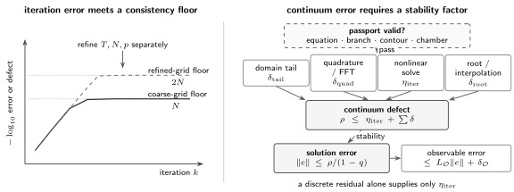
Iteration stops buying digits when it reaches the consistency floor. Branch, contour, and chamber passports must pass first; they are validity gates, not small errors. The remaining tail, quadrature, nonlinear, root, reconstruction, and arithmetic defects then receive a stability factor. The observable has its own evaluation error.

Excited roots belong to the nonlinear unknown

For the sourced equations of Page 5, solve for the field samples and root positions together:

$$U = \left( \varepsilon_{a,k}, \theta_1,\ldots,\theta_m \right).$$

Augment the field residual by

$$G_j(U) = \varepsilon_{b_j}(\theta_j) -(2I_j+1)\pi\ii =0.$$

The Newton system has the block form

$$\begin{pmatrix} A&B\\ C&D \end{pmatrix} \begin{pmatrix} \delta\varepsilon\\ \delta\boldsymbol\theta \end{pmatrix} = - \begin{pmatrix} F\\G \end{pmatrix}.$$

Here $A=I-D_\varepsilon\mathcal T$ and the root column has the sign

$$B = F_{\boldsymbol\theta} = -D_{\boldsymbol\theta}\mathcal T.$$

If the roots enter only through $S$, then $B=-\partial_{\boldsymbol\theta}S$. The remaining blocks act as

$$\delta G_j = (\delta\varepsilon_{b_j})(\theta_j) + \varepsilon_{b_j}'(\theta_j)\delta\theta_j.$$

A simple divisor requires $\varepsilon_{b_j}'(\theta_j)\neq0$. Evaluate off-grid and off-axis quantities with controlled spectral or barycentric interpolation, or directly from the integral representation. Snapping a root to the nearest real grid point changes the quantization problem.

Continuation is predictor–corrector with event detection

For $H(U,\lambda)=0$, where $H_U$ is invertible, a tangent predictor solves the Davidenko equation

$$H_U U'(\lambda) = -H_\lambda.$$

Newton then corrects the full system at the new parameter. Near a fold, replace $\lambda$ as the continuation coordinate by pseudo-arclength and realify the complex system. Using the normalized previous tangent $(t_U,t_\lambda)$ and real $\lambda$, add the one real equation

$$t_U^{\mathsf T}(U-U_0) + t_\lambda(\lambda-\lambda_0) = \Delta s.$$

Every accepted step should monitor at least

$$c_{\log} = \min_a \inf_{z\in\Gamma_a^{\mathrm{active}}} |1+\ee^{-\varepsilon_a(z)}|,$$

where the active contours exclude already declared divisor indentations. Also track each known zero’s signed normal distance to its contour, source-root separations, branch integers, a Jacobian conditioning indicator, and Page 5’s first kernel-wall functions

$$g_{ab}^{+} = \frac\pi2-(\phi_b-\phi_a), \qquad g_{ab}^{-} = \frac\pi2+(\phi_b-\phi_a).$$

If a signed pole-to-contour distance or wall function changes sign, or if $c_{\log}$ or a source-root separation falls below its alarm threshold, return to the last checkpoint and locate the event off-grid.

A grid approximation to $c_{\log}$ is only an event alarm: a zero can lie between grid points or off the real line. Before updating any Page 5 ledger, confirm the crossing by off-grid analytic zero tracking or by comparing argument-principle counts at the two bracketing checkpoints; a sampled minimum alone does not determine its orientation.

A fully converged corrector removes the predictor error only up to the discrete nonlinear tolerance; it does not remove discretization, event-detection, or branch-selection error. Repeat the path with smaller steps and test continuity of a normalization-independent observable.

The symmetric A₂ equation calibrates the real TBA discretization

Set $m_1=m_2=1$ in the real minimal $A_2$ system and impose reflection symmetry. The two equations reduce to

$$\varepsilon(\theta) = \ee^\theta - \int_{\mathbb R} \frac{ \log(1+\ee^{-\varepsilon(\theta')}) }{ 2\pi\cosh(\theta-\theta') } \dd\theta'.$$

As $\theta\to-\infty$ the drive vanishes. With $Y_-=\ee^{-\varepsilon_-}$ and $\int K=1/2$, the constant equation gives

$$Y_-^2=1+Y_-, \qquad Y_-=\frac{1+\sqrt5}{2}, \qquad \varepsilon_-=-\log Y_-.$$

This golden-ratio plateau checks the kernel normalization, nonlinear logarithm, sign, and left-tail model simultaneously.

The downloadable reference implementation uses an endpoint-weighted trapezoidal rule, integrates the constant left tail analytically, embeds the Toeplitz product in a length-$2N$ FFT, and compares that product with a dense matrix. On the recorded environment the physical-kernel dense/FFT difference was $5.55\times10^{-17}$, the asymmetric lag-order audit differed by $4.44\times10^{-16}$, and the fixed-point map converged in 26 iterations.

The following cutoff sweep keeps $h\approx1/32$. The final column compares with the script’s internal $T=20$, $N=4097$ refinement value; it is not an external exact answer.

$T$	$N$	$\varepsilon(0)$	Change from internal refinement
6	385	0.8091575433257463	$7.30\times10^{-6}$
8	513	0.8091645695094771	$2.73\times10^{-7}$
10	641	0.8091648363706210	$6.21\times10^{-9}$
12	769	0.8091648433180046	$7.41\times10^{-10}$

At fixed $T=12$, refining $N=193,385,769,1537$ changes $\varepsilon(0)$ from $0.8091648619951218$ to $0.8091648423838714$. The tiny discrete residuals, about $10^{-15}$, clearly do not equal the forward changes. Cutoff and mesh refinements reveal errors that the inner iteration cannot see.

A production report separates every control

Record a run as a refinement tuple such as

$$\mathcal R = (T_-,T_+,N,P_{\mathrm{FFT}},p, \tau_{\mathrm{NL}}, \delta_{\mathrm{bank}}, \Delta\lambda, \tau_{\mathrm{root}}),$$

where $P_{\mathrm{FFT}}$ is the FFT embedding length and $p$ the working precision. Given an observable tolerance $\tau_{\mathcal O}$, contraction allocates the approximate field-defect budget

$$\eta_{\mathrm{iter}}+\delta_{\mathrm{disc}} \leq \frac{ (\tau_{\mathcal O}-\delta_{\mathcal O})(1-q) }{L_{\mathcal O}},$$

provided $\tau_{\mathcal O}>\delta_{\mathcal O}$. Stop the nonlinear iteration once $\eta_{\mathrm{iter}}$ is safely below the dominant consistency contribution; further inner digits do not improve the target observable.

Vary one component of $\mathcal R$ at a time to identify error sources, then perform at least one combined diagonal refinement. That final run can expose cancellation between, for example, cutoff and mesh errors.

Error or failure mode	Independent control
Equation/passport	Recheck normalization, branches, sources, and chamber
Left and right tails	Increase $T_-$ and $T_+$ separately
Quadrature	Reduce $h$ or increase panel order at fixed domain
FFT wrap or lag error	Increase padding and compare a direct convolution
Nonlinear solve	Tighten the raw $F$ residual without changing the grid
Root interpolation	Increase interpolation order and evaluate off-grid
Arithmetic and conditioning	Raise precision and estimate $DF^{-1}$
Lateral prescription	Vary the bank displacement and extrapolate in its valid chart
Observable evaluation	Refine its integral independently of the field solve
Spectral root	On a real monotone bracket, divide the residual by a verified lower bound for $

Finally test identities not imposed by the solver: evaluate the continuum residual on a shifted or doubled grid, verify the original Y-system inside the safe strip, reconstruct an RH jump on both banks, recover the WKB drive or moment, test node symmetries, and compare the target observable with direct ODE data. Two implementations sharing the same FFT indexing bug are not independent checks.

Common pitfalls

Calling a small collocation residual an error bound. It controls the finite nonlinear solve. First validate the passport; then bound tail, quadrature, reconstruction, arithmetic, and stability errors.

Claiming spectral convergence across an endpoint jump. Strip analyticity does not repair a discontinuous periodization. Subtract the unequal asymptotics or use a nonperiodic rule.

Using signed kernel mass in a contraction test. Bounds require $\int|K|$, especially for complex shifted kernels. Cancellation is not a global Lipschitz certificate.

Exercises

1. Stabilize the nonlinear logarithm. Prove that for real $x$,

$$\log(1+\ee^{-x}) = \max(0,-x) + \log(1+\ee^{-|x|}),$$

and find its derivative. Why does the same rewrite need an extra integer for complex $x$?

Solution

For $x\geq0$ the maximum vanishes and the identity is immediate. For $x<0$, factor out $\ee^{-x}$:

$$\log(1+\ee^{-x}) = -x+\log(1+\ee^x).$$

In both regions,

$$\frac{\dd}{\dd x} \log(1+\ee^{-x}) = -\frac{1}{1+\ee^x}.$$

For complex $x$, factorization remains algebraically valid, but the two logarithms may differ by $2\pi\ii n$. Continuation and the declared branch, not the sign of $\Re x$ alone, determine $n$.

2. Calibrate the hyperbolic kernel. For

$$K(u)=\frac{1}{2\pi\cosh u},$$

compute its $L^1$ norm and two-sided tail mass. Then solve the constant zero-drive equation

$$\varepsilon = -K*\log(1+\ee^{-\varepsilon}).$$

Solution

Since $\int_{\mathbb R}\operatorname{sech}u\,\dd u=\pi$,

$$\|K\|_1=\frac12.$$

The antiderivative gives

$$\int_{|u|>T}K(u)\,\dd u = \frac{2}{\pi}\arctan(\ee^{-T}).$$

Put $Y=\ee^{-\varepsilon}$. Constancy of the convolution gives

$$-\log Y = -\frac12\log(1+Y),$$

so $Y^2=1+Y$. Positivity selects

$$Y=\frac{1+\sqrt5}{2}, \qquad \varepsilon=-\log\frac{1+\sqrt5}{2}.$$

This one number tests the sign, nonlinear function, and kernel normalization.

3. Recover linear convolution with an FFT. Two sampled arrays have length $N$. Explain why a transform length $P_{\mathrm{FFT}}\geq2N-1$ prevents wraparound, and identify the continuum mesh factor.

Solution

Their linear discrete convolution has indices $0,\ldots,2N-2$ and hence length $2N-1$. A length-$P_{\mathrm{FFT}}$ DFT computes indices modulo $P_{\mathrm{FFT}}$. When $P_{\mathrm{FFT}}\geq2N-1$, no two linear coefficients are identified. Embed the positive and negative kernel lags in circulant order, zero-pad the weighted data, multiply transforms, and crop the desired $N$ entries.

The inverse FFT already contains $1/P_{\mathrm{FFT}}$. The Riemann sum contributes the single additional factor $h$:

$$c_j = h\sum_k K((j-k)h)f_k.$$

Padding fixes discrete wraparound, not the omitted infinite tails.

4. Choose a mesh from strip clearance. Suppose

$$E_h \leq \frac{2B}{\exp(2\pi a/h)-1}.$$

Find a sufficient condition on $h$ for $E_h\leq\tau$. Interpret the limit $a\to0$.

Solution

It is enough that

$$\exp(2\pi a/h)-1 \geq \frac{2B}{\tau}.$$

Therefore

$$h \leq \frac{2\pi a}{ \log(1+2B/\tau) }.$$

As a kernel pole, source cut, or logarithmic divisor approaches the contour, $a$ tends to zero and the required mesh becomes arbitrarily fine. At a genuine crossing the correct response is a contour or coordinate update, not infinite refinement of the obsolete chart.

5. Turn consistency into a forward bound. Let $\mathcal T$ be a contraction with constant $q<1$, and suppose the passport gate has passed. Assume $\mathcal T$ maps a complete set $\mathscr U$ into itself. A lifted discrete map $\widetilde{\mathcal T}_N$ and continuous candidate $x\in\mathscr U$ satisfy

$$\|x-\widetilde{\mathcal T}_Nx\|\leq r, \qquad \|\widetilde{\mathcal T}_Nx-\mathcal Tx\|\leq\delta.$$

Bound its distance from the exact fixed point $x^*$. If an observable is $L_{\mathcal O}$-Lipschitz and its numerical evaluation has defect $\delta_{\mathcal O}$, also bound its forward error.

Solution

Using $x^*=\mathcal Tx^*$,

$$\begin{aligned} \|x-x^*\| \leq{}& \|x-\widetilde{\mathcal T}_Nx\| + \|\widetilde{\mathcal T}_Nx-\mathcal Tx\| \\ &+ \|\mathcal Tx-\mathcal Tx^*\|. \end{aligned}$$

Hence

$$\|x-x^*\| \leq r+\delta+q\|x-x^*\|,$$

and therefore

$$\|x-x^*\| \leq \frac{r+\delta}{1-q}.$$

The term $r$ is the nonlinear-solve defect; $\delta$ must still bound the tail, quadrature, reconstruction, controlled contour-displacement, root, and arithmetic consistency errors. The observable consequently obeys

$$|\mathcal O_{\mathrm{num}}-\mathcal O(x^*)| \leq \delta_{\mathcal O} + L_{\mathcal O}\frac{r+\delta}{1-q}.$$

6. Decide what damping can stabilize. If $\mu$ is an eigenvalue of $D\mathcal T(\varepsilon^*)$, find the corresponding eigenvalue of damped Picard iteration. Can positive damping stabilize (a) $\mu=-2$ and (b) $\mu=1.2$?

Solution

The damped linearized eigenvalue is

$$\mu_\omega = 1-\omega+\omega\mu = 1-\omega(1-\mu).$$

For $\mu=-2$, the condition $|1-3\omega|<1$ gives

$$0<\omega<\frac23.$$

Thus under-relaxation can stabilize this oscillatory mode. For $\mu=1.2$,

$$\mu_\omega=1+0.2\omega>1$$

for every positive $\omega$. Damping cannot stabilize that growing positive mode, nor does an empirical stable run replace a global norm argument.

7. Linearize an excited root. Let a sourced field equation be written as $F(\varepsilon,\theta_*)=0$ and impose

$$G(\varepsilon,\theta_*) = \varepsilon_b(\theta_*)-(2I+1)\pi\ii =0.$$

Write the Newton blocks and state the simple-root condition.

Solution

The coupled correction obeys

$$\begin{pmatrix} F_\varepsilon&F_{\theta_*}\\ G_\varepsilon&G_{\theta_*} \end{pmatrix} \begin{pmatrix} \delta\varepsilon\\ \delta\theta_* \end{pmatrix} = - \begin{pmatrix} F\\G \end{pmatrix}.$$

Since $F=\varepsilon-\mathcal T$, the root column is

$$F_{\theta_*} = -\partial_{\theta_*}\mathcal T.$$

If the root enters only through the oriented source $S$, this becomes $F_{\theta_*}=-\partial_{\theta_*}S$. The lower blocks are

$$G_\varepsilon\delta\varepsilon = (\delta\varepsilon_b)(\theta_*), \qquad G_{\theta_*} = \varepsilon_b'(\theta_*).$$

The divisor is simple when $\varepsilon_b'(\theta_*)\neq0$. A small derivative makes the root ill-conditioned and calls for off-grid analytic evaluation rather than snapping it to a node.

8. Predict the first continuation event. At $\lambda_0$, suppose

$$\Delta\phi=1.50, \qquad \frac{\dd\Delta\phi}{\dd\lambda}=0.40,$$

while

$$c_{\log}=0.08, \qquad \frac{\dd c_{\log}}{\dd\lambda}=-0.30.$$

Assuming these derivatives remain constant and the same smooth minimizer of $c_{\log}$ remains active, estimate whether the first positive kernel wall or the logarithmic-divisor alarm occurs first.

Solution

The first positive kernel wall is at $\Delta\phi=\pi/2$, so the linear prediction is

$$\Delta\lambda_K \approx \frac{\pi/2-1.50}{0.40} \approx0.177.$$

The predicted divisor clearance reaches zero after

$$\Delta\lambda_{\log} \approx \frac{0.08}{0.30} \approx0.267.$$

The kernel event is predicted first. The extrapolated zero of sampled $c_{\log}$ would only be an alarm requiring off-grid confirmation. Shorten the step, locate the kernel event, and update the contour-residue ledger. Do not add an excited root merely because another clearance is decreasing, and do not infer a BPS-index change without the separate chamber data.

References

• L. N. Trefethen and J. A. C. Weideman, “The Exponentially Convergent Trapezoidal Rule”, SIAM Review 56 (2014), 385–458, especially Theorems 3.2 and 5.1. Gives the periodic- and infinite-line strip-analytic error estimates and explains their decay and singularity hypotheses.
• K. E. Atkinson and F. A. Potra, “Projection and Iterated Projection Methods for Nonlinear Integral Equations”, SIAM Journal on Numerical Analysis 24 (1987), 1352–1373. Gives convergence results near isolated solutions for projection and iterated projection discretizations; it is not a theorem for an arbitrary TBA branch.
• D. A. Knoll and D. E. Keyes, “Jacobian-Free Newton–Krylov Methods: A Survey of Approaches and Applications”, Journal of Computational Physics 193 (2004), 357–397. Reviews matrix-free Newton–Krylov methods, globalization, and preconditioning.
• S. C. Eisenstat and H. F. Walker, “Choosing the Forcing Terms in an Inexact Newton Method”, SIAM Journal on Scientific Computing 17 (1996), 16–32. Supplies the forcing-term criteria behind the local convergence claims used here.
• H. F. Walker and P. Ni, “Anderson Acceleration for Fixed-Point Iterations”, SIAM Journal on Numerical Analysis 49 (2011), 1715–1735. Analyzes Anderson acceleration, its quasi-Newton/secant interpretation, and its linear-problem relation to GMRES; it does not make a branch-incorrect fixed point physically valid.
• H. B. Keller, “Numerical Solution of Bifurcation and Nonlinear Eigenvalue Problems,” in P. H. Rabinowitz (ed.), Applications of Bifurcation Theory, Publication of the Mathematics Research Center 38, Academic Press, 1977, 359–384. Develops the pseudo-arclength continuation framework used in the predictor–corrector discussion.
• L. M. Delves and J. N. Lyness, “A Numerical Method for Locating the Zeros of an Analytic Function”, Mathematics of Computation 21 (1967), 543–560. Develops argument-principle contour methods useful for checking complex source roots and collisions.
• P. Dorey and R. Tateo, “Excited States by Analytic Continuation of TBA Equations”, Nuclear Physics B 482 (1996), 639–659, especially §2. Uses damped iteration, small continuation steps, zero tracking, and contour deformation, while explicitly reporting the limitations of the numerical iteration.
• K. Ito, M. Mariño, and H. Shu, “TBA Equations and Resurgent Quantum Mechanics”, Journal of High Energy Physics 2019 (2019), 228, especially §§4–5. Implements Fourier discretizations and independent spectral or WKB checks; its reported high-resolution computations and independent comparisons are strong evidence rather than universal certified bounds.
• D. Gaiotto, G. W. Moore, and A. Neitzke, “Four-Dimensional Wall-Crossing via Three-Dimensional Field Theory”, Communications in Mathematical Physics 299 (2010), 163–224, especially Appendix C. Establishes contraction of successive RH iterates in a sufficiently large-$R$ regime under support and growth assumptions; it does not certify an arbitrary floating-point discretization.
• NIST Digital Library of Mathematical Functions, §3.5, “Quadrature”. An official overview of classical quadrature rules, error terms, and practical qualifications.